Deep MIB - Train tab
This tab contains settings for generating deep convolutional network and training.
Back to Index --> User Guide --> Menu --> Tools Menu --> Deep learning segmentation
Contents
-
Train tab -
Network design -
Augmentation design -
Training process design -
Start the training process
Train tab
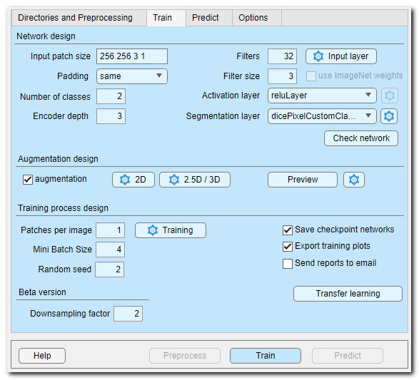
Before starting the training process it is important to check and adapt
the default settings to needs of the specific project.
As the starting point make sure the name of the output network is selected using
the Network filename button of the Network
panel.
Network design
The Network design section is used to set the network configuration settings. Please check the following list to understand details of available configuration options.

Widgets of the Network design section
- Input patch size..., this is an important field that has to be defined
based on available memory of GPU, desired size of image area that network can see at once, dimensions of the training dataset and
number of color channels.
The input patch size defines dimensions of a single image block that will be directed into the network for training. The dimensions are always defined with 4 numbers representing height, width, depth, colors of the image patch (for example, type "572 572 1 2" to specify a 2D patch of 572x572 pixels, 1 z-slice and 2 color channels).
The patches are taken randomly from the volume/image and number of those patches can be specified in the Patches per image... editbox. - Padding ▼ defines type of the convolution padding, depending on
the selected padding the Input patch size may have to be
adjusted; use the Check network button to make
sure that the input patch size is correctly matching the selected padding.
- same - zero padding is applied to the inputs to convolution layers such that the output and input feature maps are the same size
- valid - zero padding is not applied to the inputs to convolution layers. The convolution layer returns only values of the convolution that are computed without zero padding. The output feature map is smaller than the input feature map. Valid padding in general produces results with less edge artefacts, but the overlap prediction mode for Same padding is capable to also minimize the artefacts.
- Number of classes... - number of materials of the model including Exterior, specified as a positive number
- Encoder depth... - number of encoding and decoding layers of the
network. U-Net is composed of an encoder subnetwork and a corresponding decoder subnetwork.
The depth of these networks determines the number of times the input image is
downsampled or upsampled during processing. The encoder network downsamples
the input image by a factor of 2^D, where D is the value of EncoderDepth.
The decoder network upsamples the encoder network output by a factor of 2^D.
The Downsampling factor... editbox in the Beta version can be used to tweak the downsampling factor to increase the input patch size so that network sees a larger area. - Filters... - number of output channels for the first encoder stage, i.e. number of convolitional filters used to process the input image patch during the first stage. In each subsequent encoder stage, the number of output channels doubles. The unetLayers function sets the number of output channels in each decoder stage to match the number in the corresponding encoder stage
- Filter size... - convolutional layer filter size; typical values are 3, 5, 7
- The Input layer button - press to specify settings for normalization of images during training.
- [✓] use ImageNet weights (only for MATLAB version of MIB), when checked the networks of the 2D patch-wise workflow are initialized using pretrained weights from training on more than a million images from the ImageNet database This requires that supporting packages for the corresponding networks are installed and allows to boost the training process significantly
- Activation layer ▼ - specifies type of the activation layers of
the network. When the layer may have additional options, the settings
button
 on the right-hand side becomes available.
List of available activation layers
- reluLayer - Rectified Linear Unit (ReLU) layer, it is a default activation layer of the networks, however it can be replaced with any of other layer below
- leakyReluLayer - Leaky Rectified Linear Unit layer performs a threshold operation, where any input value less than zero is multiplied by a fixed scalar
- clippedReluLayer - Clipped Rectified Linear Unit (ReLU) layer performs a threshold operation, where any input value less than zero is set to zero and any value above the clipping ceiling is set to that clipping ceiling
- eluLayer - Exponential linear unit (ELU) layer performs the identity operation on positive inputs and an exponential nonlinearity on negative inputs
- swishLayer - A swish activation layer applies the applies the swish function (f(x) = x / (1+e^(-x)) ) on the layer inputs
- tanhLayer - Hyperbolic tangent (tanh) layer applies the tanh function on the layer inputs
- Segmentation layer ▼ - specifies the output layer of the
network; depending on selection the settings button
 on the right-hand side
becomes available to bring access to additional parameters.
List of available segmentation layers
- pixelClassificationLayer - semantic segmentation with the crossentropyex loss function
- focalLossLayer - semantic segmentation using focal loss to deal with imbalance between foreground and background classes. To compensate for class imbalance, the focal loss function multiplies the cross entropy function with a modulating factor that increases the sensitivity of the network to misclassified observations
- dicePixelClassificationLayer - semantic segmentation using generalized Dice loss to alleviate the problem of class imbalance in semantic segmentation problems. Generalized Dice loss controls the contribution that each class makes to the loss by weighting classes by the inverse size of the expected region
- dicePixelCustomClassificationLayer - a modification of the dice loss, with better control for rare classes
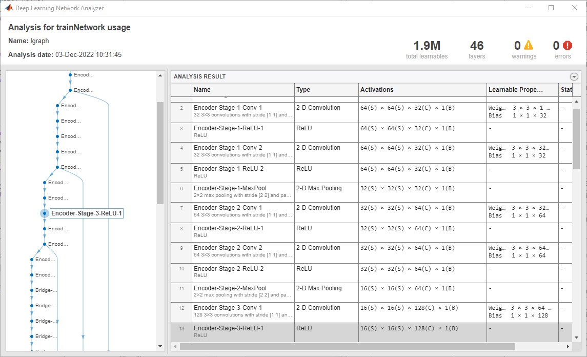
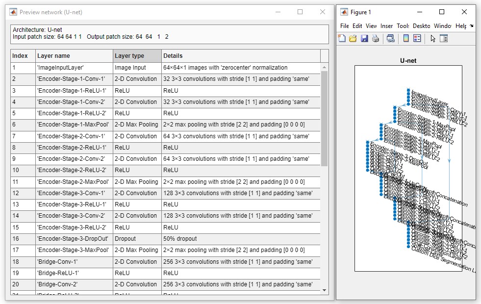
- Check network - press to preview and check the network. The standalone version of MIB shows only limited information about the network and does not check it.
Snapshots of the network check window for the MATLAB and standalone versions of MIB
A snapshot of the network check preview for the MATLAB version of MIB:
A snapshot of the network check preview for the standalone version of MIB:
Augmentation design
Augmentation of the training sets is an easy way to extend the training base by applying variouos image processing filters to the input image patches. Depending on the selected 2D or 3D network architecture a different sets of augmentation filters are available (17 for 2D and 18 for 3D).

These operations are configurable using the 2D and 3D settings buttons on the right-hand side from the [✓] augmentation checkbox
It is possible to specify percentage of image patches that are going to be augmented and each augmentation can be fine tuned by providing its probability and its variation. Note that an image patch may be subjected to multiple augmentation filters at the same time, depending on their probability factor.
- [✓] Augmentation - augment data during training. When this checkbox is checked the input image patches are additionally filtered with number of defined filters. The exact augmentation options are available upon hitting the 2D and 3D buttons
- 2D - press to specify augmentation settings for 2D networks. There are 17 augmentation operations and it is possible to specify fraction of images patches that have to be augmented and set variation and probability for each augmentation filter to be triggered. Expand the following section to learn about 2D/3D augmentation settings.
- 3D - press to specify augmentation settings for 3D networks. There are 18 augmentation operations and it is possible to specify fraction of images patches that have to be augmented and set variation and probability for each augmentation filter to be triggered. Expand the following section to learn about 2D/3D augmentation settings.
2D/3D augmentation settings
Upon pressing of the 2D or 3D buttons, a dialog will be displayed that provides access to select augmentation settings.
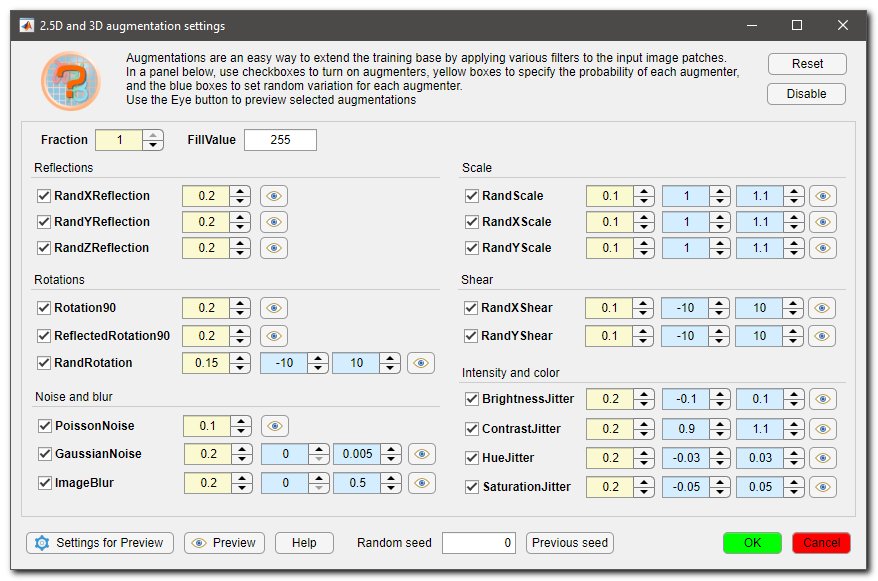
Each augmentation may be can be toggled on or off using a checkbox next to its name. Additionally it is possible to specify the probability for each augmentation to be triggered using yellow spinboxes (probability), as well as their variation range using light blue spinboxes (variation).
The augmentation settings can be reset to their default states by clicking the Reset button or disabled altogether using the Disable button.
- Fraction allows you to specify the probability that a patch will be augmented. When set to Fraction==1 all patches are augmented using the selected set of augmentations. When set to Fraction==0.5 only 50% of the patches will be augmented.
- FillValue allows you to specify the background color when patches are downsampled or rotated. When FillValue==0 the background color is black, when FillValue==255 the background color is white (for 8-bit images)
 use these
checkboxes to toggle augmentations on and off
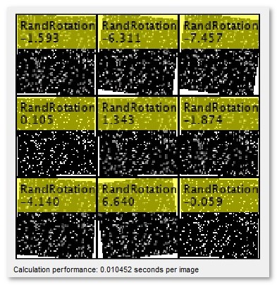
 is used to preview input image patches that are
generated using augmentor. It is useful for evaluation of augmenter
operations and understanding performance. Depending on a value in
Radnom seed the same (when set to "0") or a random image patch will be used
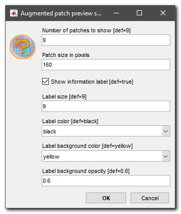
 allows to specify
parameters used to preview the augmentations.
Details settings for preview
Snapshot of settings to preview the selected augmentation operations:
Example of augmentations generated by press of the Preview button:
- Help press to jump to the Training details section of the help system
- Random seed when set to "0" a random patch is shown each time the augmentations are previews, when set to any other number a fixed random patch is displayed
- Previous seed when using a random seed (Random seed==0) you can restore the previous random seed and populate the Random seed with it. When done like that, the preview patches will be the same as during the previous preview call
- OK press to accept the current set of augmentations and close the dialog
- Cancel, close the dialog without accepting the updated augmentations
Training process design
In this section a user can specify details on of the training process that is started upon press of the Train button.
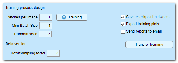
Widgets of the Training process design section
- Patches per image... - specify number of image patches that will be taken from each an image or a 3D dataset at each epoch. According to our experience, the best strategy is to take 1 patch per image and train network for larger number of epochs. When taking a single patch per image it is important to set Training settings (Training button)->Shuffling->every-epoch). However, fill free to use any sensible number
- Mini Batch Size... - number of patches processed at the same time by the network. More patches speed up the process, but it is important to understand that the resulting loss is averaged for the whole mini-batch. Max number of mini batches is limited by available GPU memory
- Random seed... set a seed for a random number generator used during initialization of training. We recommend to use a fixed value for reproducibility, otherwise use 0 for random initialization each time the network training is started
- Training - define multiple parameters used for training, for details please refer to
trainingOptions
function
Tip, setting the Plots switch to "none" in the training settings may speed up the training time by up to 25%
- [✓] Save checkpoint networks when ticked DeepMIB
saves the training progress in checkpoint files after each epoch to
3_Results\ScoreNetwork directory.
It will be possible to choose any of those networks and continue training from that checkpoint. If the checkpoint networks are present, a choosing dialog is displayed upon press of the Train button.
In R2022a or newer it is possible to specify frequency of saving the checkpoint files. - [✓] Export training plots when ticked accuracy and loss scores are saved to 3_Results\ScoreNetwork directory. DeepMIB uses the network filename as a template and generates a file in MATLAB format (*.score) and several files in CSV format
- [✓] Send reports to email when
ticked information about progress and finishing of the training run is
sent to email. Press on the checkbox starts a configuration window to
define SMTP server and user details
Configuration of email notifications
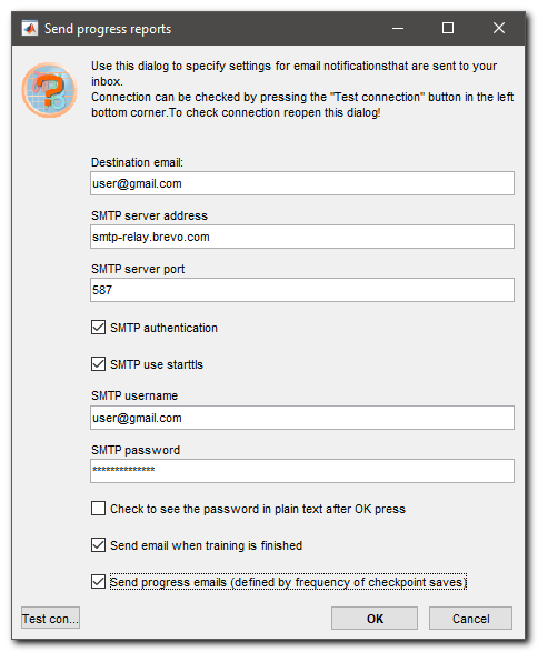
Check below the configuration settings for sending email with the progress information of the run.
Important!
Please note that the password for the server is not encoded in any way and stored in the configuration file. Do not use your email account details, but rather use a dedicated services that are providing access to SMTP servers!
For example, you can use https://www.brevo.com service that we've tested.
Configuration of brevo.com SMTP server
- Open https://www.brevo.com in a browser and Sign up for a free account
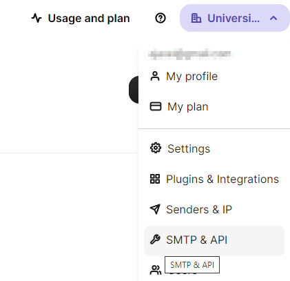
- Open the SMTP and API entry in the top right corner menu:
- Press the Generate a new SMTP key button to generate a new password to access SMTP server
- Copy the generated pass-key into the password field in the email configuration settings. You can also check the server details on this page
- Destination email, provide email address to which the notifications should be addressed
- STMP server address, address of SMTP server that will be used to send notifications
- STMP server port, port number on the server
- [✓] STMP authentication, checkbox indicating that the authentification is required by the server
- [✓] STMP use starttls, checkbox indicating that the server is using secure protocol with Transport Layer Security (TLS) or Secure Sockets Layer(SSL)
- STMP username, username on the STMP server, a user's email for brevo.com
- STMP password, password to access the server. You can use this field to type a new password; the password is hidden with ****, if you want to see it check [✓] Check to seethe password in plain text after OK press
- [✓] Send email when training is finished, when checked, an email is send at the end of the training run
- [✓] Send progress emails, when checked, emails with the progress of the run are sent with frequency specified in the checkpoint save parameter (only for the custom training dialog
- Test connection, it is highly recommended to test connection. To do that press OK to accept the settings; reopen this dialog and press Test connection
Start the training process
To start training press the Train button highlighted under the
panel. If a network file already exists under the provided Network filename...
it is possible to continue training from that point
(a dialog with possible options appears upon restart of training). After
starting of the training process a config file (with *.mibCfg) is created
in the same directory. The config file can be loaded from Options
tab->Config files->Load
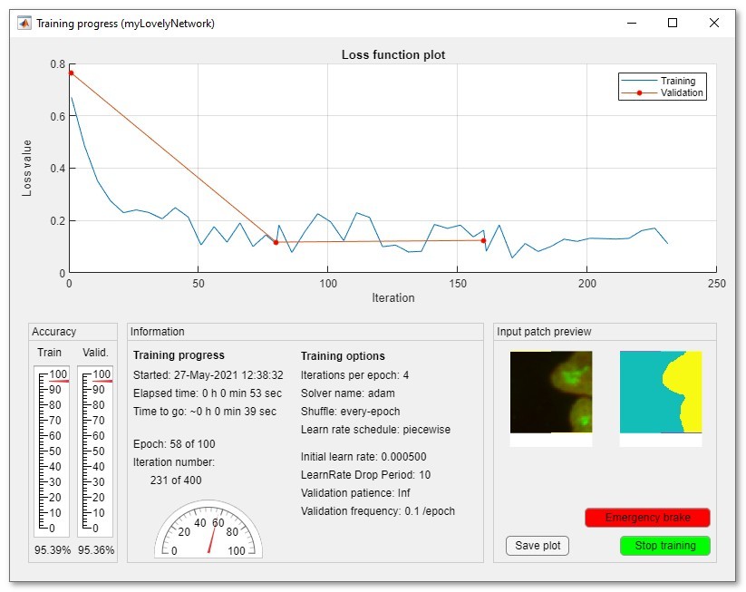
Upon training a plot with the loss function is shown; the idea of the
training is to minimize the loss function as much as possible. The blue
curve displays the loss function calculated for the train set, while the
red curve for the validation set. The accuracy of the prediction for both
train and validation sets is displayed using the linear gauge widgets at
the left bottom corner of the window.
right mouse click over the plot opens a popup menu, that can be
used to scale the plot.
It is possible to stop training at any moment by pressing the Stop or
Emergency brake buttons. When the Emergency brake button
is pressed DeepMIB will stop the training as fast as possible, which may lead to
not finalized network in situations when the batch normalization layer is
used.
Please note that by default DeepMIB is using a custom progress plot. If you want to use
the progress plot provided with MATLAB (available only in MATLAB version
of MIB), navigate to Options tab->Custom training plot->Custom
training progress window: uncheck
The plot can be completely disabled to improve performance:
Train tab->Training->Plots, plots to display during network
training->none
The right bottom corner of the window displays used input image and model
patches. Display of those decreases training performace, but the frequency
of the patch updates can be modified in Options tab->Custom training
plot->Preview image patches and Fraction of images for preview. When
fraction of image for preview is 1, all image patches are shown. If the value
is 0.01 only 1% of patches is displayed.
After the training, the network and config files with all paramters are generated in location specified in the
Network filename... editbox of the Network panel.
Back to Index --> User Guide --> Menu --> Tools Menu --> Deep learning segmentation