3D-Modeling with Microscopy Image Browser (im_browser)
(pdf version)
Ilya Belevich, Darshan Kumar, Helena Vihinen
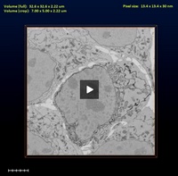
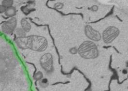
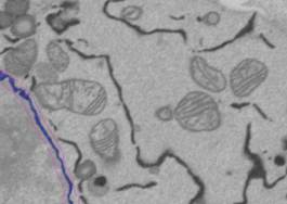
Dataset: Huh7.tif (original), obtained by Serial Block Face-SEM (Gatan 3View)
Huh7_crop.tif (cropped)
Dimensions: 32.58 x 32.58 x 2.22 μm (original)
7.01 x 4.99 x 2.22 μm (cropped)
Pixel size: 13.45 x 13.45 x 30 nm
Link to the dataset (12 Mb):
https://www.mv.helsinki.fi/home/ibelev/projects/im_browser/tutorials/3D_Modeling_files/Huh7.tif
Link to the model (0.5 Mb):
https://www.mv.helsinki.fi/home/ibelev/projects/im_browser/tutorials/3D_Modeling_files/Model.mat
A similar tutorial in 8 parts is also available on the MIB video channel on youtube.com:
Check and tune default settings of im_browser to own preferences:
Open the Preferences window (Menu->File->Preferences) and modify default parameters:
1. Define the mouse wheel action: by default, the mouse wheel is used to change slices and the "Q"/"W" keyboard buttons are used to zoom in/out. It is possible to swap these actions from the Preferences menu (Mouse wheel -> zoom). When the mouse wheel mode is set on zoom, the zoom in/out can be done with the mouse wheel and changes to the slices are done with the "Q"/"W" buttons.
2. Define the left mouse button action: by default, the left mouse button is responsible for selection (i.e., drawing using the Brush tool) and the right mouse button is used for moving the image left/right and up/down. The mouse button actions can also be swapped in the Preferences dialog (Left Mouse Button -> pan).
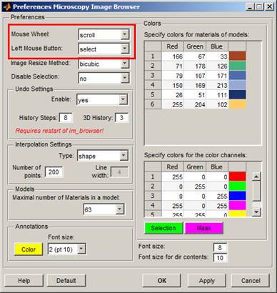
3. It is possible to set the other parameters, such as colors for materials of models and image color channels, the type of the interpolator and its settings, length of undo history, etc...
Note! The mouse wheel and buttons actions can also be set from buttons in the toolbar of im_browser.
Modeling part
I. Find and load the dataset
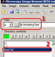 Select
the logical drive where the Huh7.tif file is stored (the link to this
dataset is in the header of this page) and navigate to the directory using the
list box in the Directory Contents Panel. Double click on a file to open
it.
Select
the logical drive where the Huh7.tif file is stored (the link to this
dataset is in the header of this page) and navigate to the directory using the
list box in the Directory Contents Panel. Double click on a file to open
it.
II. Normalize layers
This step is not always needed, but such normalization may be used to better unify the intensities of objects. Menu->Image->Contrast->Normalize layers.
III. Start a new model
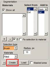 This
can be done from the im_browser menu (Menu->Models->New model) or
by pressing the Create button in the Segmentation
Panel.
This
can be done from the im_browser menu (Menu->Models->New model) or
by pressing the Create button in the Segmentation
Panel.
IV. Add a material to a model
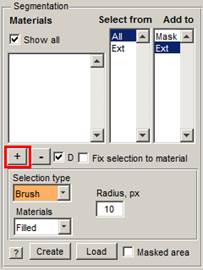 The
model consists of materials. For example, materials for cells may include mitochondria,
a nuclear envelope, plasma membrane, endoplasmic reticulum, etc. The
material called Ext - is a background (exterior). Each pixel of
the dataset can belong to only one material, so it is not possible to have two
materials above the same pixel.
The
model consists of materials. For example, materials for cells may include mitochondria,
a nuclear envelope, plasma membrane, endoplasmic reticulum, etc. The
material called Ext - is a background (exterior). Each pixel of
the dataset can belong to only one material, so it is not possible to have two
materials above the same pixel.
Press the "+" button in the Segmentation panel to add a new material. The new material, assigned as 1, will appear in the Materials, Select from and Add to lists. It is possible to remove a material from the model by selecting the material from the Select from list and pressing the "-" button.
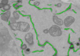
V. Trace out the nuclear envelope (NE)
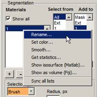 1.
Set a name for the first material in the model: In
the Materials list, select material 1, press the right mouse
button, and select Rename. Name this material as NE - the nuclear
envelope
1.
Set a name for the first material in the model: In
the Materials list, select material 1, press the right mouse
button, and select Rename. Name this material as NE - the nuclear
envelope
2. Select the Brush tool: Segmentation Panel->Selection type->Brush.
Note: Alternatively, it is possible to use the Membrane ClickTracker tool (Segmentation Panel->Selection type-> Membrane ClickTracker). Set the width to 10 and press the Shift+left mouse button to define the beginning of a membrane profile; press the left mouse button again at the end of the membrane profile. The ClickTracker traces the membrane from the starting to the ending point. If tracing fails, press Ctrl+Z to Undo the tracing and place the second point closer to the starting point. For the Linux distribution it may be required to compile the corresponding function, otherwise the performance of the ClickTracker will be too slow (please refer to the System requirements section of the im_browser Help).
3. Select slice 1 with a slider or the corresponding edit box in the Image View panel.
4.
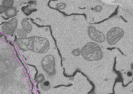
4. Draw a line with a brush (or use the Membrane ClickTracker tool) (size 10) above the NE (press and hold the left mouse button to draw, or hold the Ctrl key together with the left mouse button to erase). At this point we are not interested in an exact tracing of NE; instead, we want to make a rough mask around it.
Note: the size of the Brush can be regulated with the mouse wheel: hold the Ctrl key and use the mouse wheel to set the desired size of the Brush.
5. Repeat the drawing for each ~7-8th slice.
6. Now interpolate the drawn profiles and fill the gaps between the slices. To accomplish this, we need to check the settings of the line interpolator (Menu->File->Preferences->Interpolation Settings):
1.
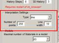 Set Type to Line
2. Set the number of points to 250 (more points provide better results but increase computation time)
3. Set the line width: to match our brush size -> 10
The type of the interpolator (line or shape) can also be selected using the corresponding button in the toolbar.
Interpolate the selection (Menu->Selection->Interpolate, or 'i' shortcut). This will use linear interpolation to complement the selection to all slices.
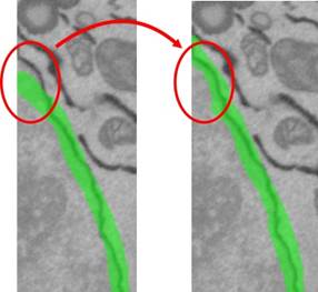
7. Go through slices to check the result of the Interpolation procedure; use the brush tool for fine tuning.
8. Set
selection as the mask: select Segmentation Panel->Add to->Mask.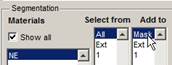
Press 'Shift + R' or Menu->Selection->...->Mask->All frames->Replace.
9. Threshold the nuclear envelope.
1. Select the BW Thresholding tool (Segmentation Panel->Selection type->BW Thresholding).
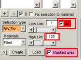 2. Select
the Masked area checkbox in the Segmentation
panel to limit thresholding only for the masked areas. Note! Please
remember that the Masked area checkbox affects all segmentation tools and you
should remember to uncheck it later!
2. Select
the Masked area checkbox in the Segmentation
panel to limit thresholding only for the masked areas. Note! Please
remember that the Masked area checkbox affects all segmentation tools and you
should remember to uncheck it later!
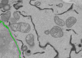
3. Move the LowLim and HighLim sliders to get a nice NE. Please note that there are some nuclear pores (for example, in slice 9) that should not be selected by threshold. Gray values: 0 and 125 should work fine. Note! It is possible to modify the sensitivity of the sliders; use the right mouse button above the slider to set its step.
4. When the proper gray levels are chosen, please select the 'all' checkbox to perform thresholding for all slices.
5. Uncheck the Masked area checkbox.
10. Add selection to the NE material of the model.
Set the target material: Segmentation Panel->Add to->1 and press 'Shift+A' (to add selection to the specified material) or 'Shift+R' buttons (to replace the material with the current selection) for all slices. It is possible to use Replace because the NE material is empty.
 R
R
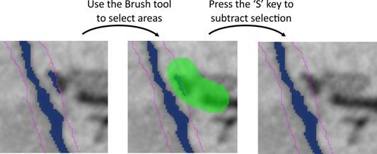
11. There may be some extra objects that do not belong to the nuclear envelope. These can be removed:
A) manually slice by slice with the brush tool: removal from the model object occurs by pressing the 'S' or 'Shift+S' (for all slices) shortcuts.
B) with object statistics/quantification:
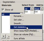
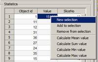
- Segmentation Panel->Materials->highlight the NE.
- press the right mouse button above 'NE' and select Get statistics... in the popup menu.
- In the appearing Material "NE" statistics... window, select Detect Objects->3D objects and press the Run button. It returns a list of areas for 3D objects that form the "NE" material of the model.
4.
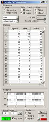
- Select the largest 3D object (object 1), press the right mouse key, and choose New selection from the popup menu to generate the new selection that highlights the largest 3D object in the Image View panel. Replace the NE material with the new selection (press 'Shift+R; you may need to click on the title bar of the main window to use the shortcut).
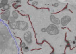
VI. Trace out the endoplasmic reticulum (ER)
1. Apply the anisotropic diffusion filter to the dataset. Anisotropic diffusion reduces local noise while preserving the edges of the structures; this usually makes the segmentation easier. Select Directory contents -> Image Filters -> Filter-> Perona Malik anisotropic diffusion. Use the following parameters: Iter: 10; K: in range from 5 to 10; lambda: 0.25; Type: Regions; the 'all' checkbox checked. Press the Filter button.
2. Remove NE from the image. To simplify the modeling we can now remove NE intensities from the dataset.
- Segmentation Panel->Select from->Highlight object 1; right mouse click to see popup menu.
-Select the NEW Selection (ALL) option to select NE for all layers of the dataset.
- Set the Strel size to 4 (Selection Panel->Strel edit box).
- Press Shift+X or the Di button in the Selection panel to dilate the selection for all layers. Using this we expand NE for 4 pixels to eliminate their dark halos.

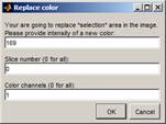 - Replace
the dataset in the selected areas with the background intensity: Menu->Selection->Replace
selected area in the image; Set intensity to 169, Slice number to 0, leave the
color channel as 1.Press OK.
- Replace
the dataset in the selected areas with the background intensity: Menu->Selection->Replace
selected area in the image; Set intensity to 169, Slice number to 0, leave the
color channel as 1.Press OK.
- Clear selection by pressing 'Shift+C".
3. Threshold ER. Add material to the model: Segmentation Panel->+ and rename it as ER.
Option 1. Manual thresholding with the Magic Wand tool.
 - Select
Segmentation panel->Selection type->Magic Wand.
- Select
Segmentation panel->Selection type->Magic Wand.
- Set threshold variation to 128 and 1. This will ensure that the Magic Wand takes only pixels that are darker than the one that has been clicked.
- Select connect 8 or 4 for detection of the connected components.
- Click on the brightest spot of the ER profile to select it.
- Hold the 'Shift' button while clicking to add the next component to the selection.
Note: The selection using the Magic Wand tool may also be done in 3D, if the Selection Panel->3D checkbox is selected.
Option 2. Local back-and-white thresholding as was used for NE. First, draw a rough mask with the brush tool and interpolate (using the Shape interpolator), and then threshold it with the Segmentation panel->Selection type->BW Thresholding. This is usually much faster than Option 1, especially in the less dense areas of the cell.
Option 3. Global black-and-white thresholding. If the ER intensities are different from the intensities of all other organelles and is more or less constant, it may be subject to global thresholding. This is the fastest way but usually produces some artifacts that have to be cleaned. Segmentation panel->Selection type->BW Thresholding. Remember to uncheck the 'Masked area' checkbox. For example, thresholding with coefficients 0 and 122 also selects some lipid bodies and bits of mitochondria.
Option 4. More sophisticated filtering.
- Select the Mask generators option in the lower right combo box of the Directory Contents panel.
- Select Mask generators->Frangi filter->Range: '1-3', Ratio: '1'; beta1: '0.9', beta2: '15', B/W Threshold: '0.3', Object size limit: '5', Black on White 'ON', All 'ON'. Do the filter (the Do It button)...
- Change the dataset plane to ZX (the ZX button in the toolbar), change the B/W Threshold to '0.38', right mouse click on the Do It button, and select Generate a new mask and add it to the existing mask. The Frangi filter detects tubular structures and cannot detect ER sheets, but this can be fixed by combining Frangi masks obtained for the different planes of the dataset.
- Repeat for the ZY plane.
In general, the results look good except a few areas at the borders of the dataset. Select the mask and assign it to the ER material of the model:
- Segmentation Panel -> Add to -> '2'.
- Select the Mask layer. Menu->Mask->...->Selection->All Frames->Replace .
- Add to ER material: 'Shift+A'.
We can rapidly add missing parts or remove something that is wrong using the Magic Wand tool (See Option 1). Ensure that the Segmentation Panel->Select from is 'Ext', Add to is '2', and the Fix selection to material is checked. When the Fix selection to material checkbox is selected, the selection is limited only to the material that is highlighted in the Select from list.
Use statistics/quantification to filter out small objects.
- Segmentation Panel->Materials -> 'ER'-> right mouse button, Get statistics....
- Set Detect Objects -> 3D objects.
- Press the Run button.
- Remove 3D objects that are smaller than 400:
- Highlight range->1-400, press the Do button
- or, using the mouse, highlight desired rows in the Statistics table and press the right mouse button to select the highlighted objects
- Uncheck Fix selection to material checkbox in the Segmentation Panel.
- Make sure that Add to is not set to Mask.
- press 'Shift+S' to subtract the selected objects from the model.
4. Remove ER from the dataset.
- Segmentation Panel->Select from -> '2'->right mouse button->New Selection (ALL) in the popup menu.
- Selection panel->Strel: '3', press 'Shift+X' to dilate the selection for all slices of the dataset. Using this, we expand ER for 3 pixels to eliminate dark halo around it.
- Menu->Selection->Replace selected area in the image: New color: 169, Slice number: 0, color channel: 1.
- Press 'Shift+C' to clear the selection layer.
VII. Trace out the lipid bodies
After the removal of ER, it is much easy to trace all other organelles.
1. Add a new object to the model: Segmentation panel->the + button and rename it as "LD".
2. Use Magic Wand in 3D to select the lipid bodies.
- Select the Magic Wand tool (Segmentation Panel->Selection type->Magic Wand.
- Set thresholds for the magic wand as 60-0.
- Set the 3D switch to ON (Selection Panel->3D) to allow selection in 3D.
- Segmentation panel-> Select from -> 'Ext'; Add to -> '3'; Fix selection to material: 'on'.
- Click with the mouse button on the lipid body outlines in its lightest point to select lipid droplets.

3. Fill the contents of the lipid bodies with 'Shift+F' shortcut, or by holding the "Shift" button and clicking on the "F" button of the Selection panel.

4. Perform erosion and dilation to remove artifacts: Select Selection Panel->3D, Strel: '4', Press the 'z' button to erode in 3D and then the 'x' button to restore the original shape.
5. Add it to the LD material object in the model: Segmentation Panel: Fix selection to material: "OFF", Add to: 3, press Shift+A.
5. Remove the lipid bodies from the dataset, similar to removal of ER.
- Segmentation Panel->Select from '3'->right mouse button->New Selection (ALL) in the popup menu.
- Selection panel->Strel: '3', press 'X' to dilate the selection for all slices of the dataset; this expands LD for 3 pixels to eliminate the surrounding dark halo.
- Menu->Selection->Replace selected area in the image: New color: 169, Slice number: 0, color channel: 1.
- Press 'Shift+C' to clear the selection layer.
6. There are some lines still present after subtraction of the ER. These lines may be removed with bottom-hat filtering. Menu->Image->Bottom-hat filtering->add to the image->Strel size: '2', Multiply result by: '1', Frames: '1:75', Smoothing, width: '0'.
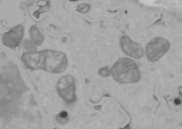
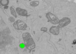
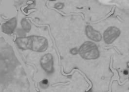
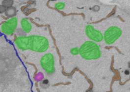
VIII. Trace out the mitochondria
1. Add a new object to the model. Segmentation panel->the + button and name it "Mitochondria".
2a. The mitochondria may be traced, for example, using brush and interpolation to create rough outlines and then local thresholding (similar to the tracing of NE, see above).
- Use the brush tool to draw a contour around mitochondria.
- Fill it with the 'F' shortcut.
- Draw the next contour after 5-6 slices and fill it...
- After one single mitochondria is outlined in this way, interpolate the shapes with the 'i' shortcut (or Menu->Selection->Interpolate) and add them to the 'Mask' layer (set Segmentation panel->Add to->Mask, press 'Shift+A' to add or "Shift+R" to replace the existing mask).
- Threshold mitochondria with Segmentation panel->Selection type->BW Thresholding. Set the Masked area and the all checkboxes to 'ON' and threshold using values '100' and '155'. At the end fill mitochondria with 'Shift+F'.
2b. The alternative way to segment mitochondria is to make global black-and-white thresholding:
- Segmentation Panel->Selection type->BW Thresholding->LowLim: 100, HighLim: 155, all: ON.
- Fill the holes with Shift+F.
- Manually draw borders around mitochondria that were not filled and fill the holes again with Shift+F.
- Erode the selected mitochondria in 3D to remove small objects: Selection Panel->3D: ON, Strel: 5, press 'Z'.
- Dilate by pressing 'X'.
- Add result to mask: Segmentation Panel->Add to->Mask, press Shift+R.
- Use mask selection in 3D to pick the mitochondria from the mask: Segmentation Panel->Selection type: Mask/Model, unselect the Model checkbox to allow selection from the Mask layer.
- press the "Recalc." button to get 3D statistics for mask objects and perform selection with the left mouse button. The selected objects may be unselected using Ctrl+mouse click.
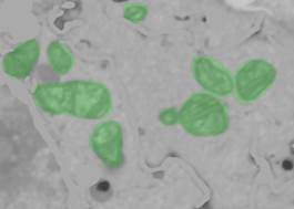
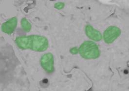
3. Add mitochondria to object 4 (Segmentation Panel->Add to->4, press Shift+A).
IX. Save the model
Menu->Models->Save Model as... save it in Matlab (*.mat) format for future use.
It is also possible to save models in several other formats, but that is recommended only for export purposes because not all these formats can be imported back into im_browser.
- Amira Mesh binary for export to Amira (*.am)
- Contours (*.mod) for IMOD
- Volumes (*.mrc) for IMOD
- NRRD format (*.nrrd) for 3D slicer
- TIF format (*.tif)
X. Visualization
Please refer to the visualization with Microscopy Image Browser for details of visualization of the models.