Deep MIB - Predict tab
This tab contains parameters used for efficient prediction (inference) of images and generation of semantic segmentation models.
Back to Index --> User Guide --> Menu --> Tools Menu --> Deep learning segmentation
Contents
-
How to start the prediction (inference) process -
Settings sections -
Explore activations -
Preview results section
How to start the prediction (inference) process
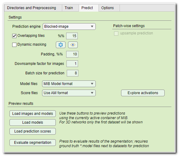
Prediction (inference) requires a pretrained network, if you do not have the pretrained network, you neet to train it.
The pretrained networks can be loaded to DeepMIB and used for prediction of new datasets
To start with prediction:
- select a file with the pretrained network in
the Network filename... editbox of the Network panel. Upon
loading, the corresponding fields of the Train panel will be
updated with the settings used for training of the loaded network
Alternatively, a config file can be loaded using Options tab->Config files->Load - make sure that directory with the images for prediction is correct
Directories and Preprocessing tab->Directory with images for prediction - make sure that the output directory for results is correct:
Directories and Preprocessing tab->Directory with resulting images - if needed, do file preprocessing (typically it is not needed):
- select Preprocess for: Prediction ▼ in the Directories and Preprocessing tab
- press the Preprocess button to perform data preprocessing
- finally switch back to the Predict tab and press the Predict button
Settings sections
The Settings section is used to specify the main parameters using for the prediction (inference) process
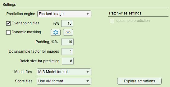
- Prediction engine ▼, use this dropdown to select a tiling engine that will be used during the prediction process. The legacy engine was in use until MIB version 2.83, for all later releases the Blocked-image engine is recommended. Some of operations (for example, Dynamic masking or 2D Patch-wise) are not available in the Legacy engine.
- [✓] Overlapping tiles, available for Padding: same ▼ convolutional padding. During prediction the edges of the predicted patch are cropped improving the segmentation, but taking more time. The percentage of the overlap between tiles can be specified using the %%... editbox.
Overlapping vs non-overlapping mode
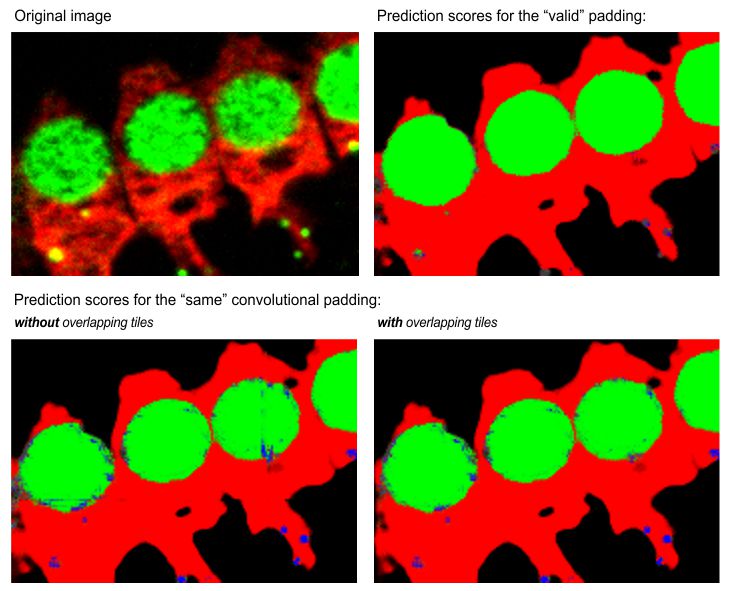
Same padding in the non-overlapping mode may have vertical and horizontal artefacts, that are eliminated when the overlapping mode is used.
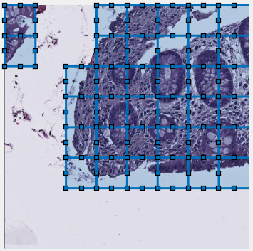
- [✓] Dynamic masking, apply on-fly masking to skip prediction on some of the tiles. Settings for dynamic masking can be specified using the Settings button on the right-hand side of the checkbox. See the block below for details.
Dynamic masking settings and preview
 , press the
button to specify parameters for dynamic masking.
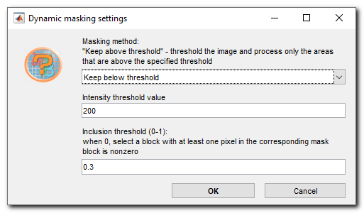
- Masking method ▼, specify whether to keep blocks with average intensity below or above the specified in the Intensity threshold value... editbox
- Intensity threshold value... is used to specify the treshold value; patches with average intensity above or below this value will be predicted
- Inclusion threshold (0-1)... is used to specify a fraction of pixels that should be above or below the tresholding value to keep the tile for prediction
- The Eye button, hit to see the effect of the specified dynamic masking settings on a portion of the image that is currently shown in the Image View panel of MIB
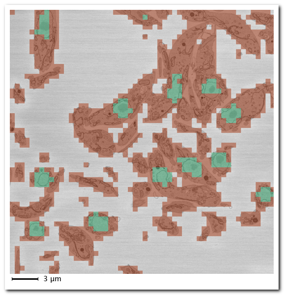
Example of patch-wise segmentation with dynamic masking
Snapshot showing result of 2D patch-wise segmentation of nuclei.
- Green color patches indicate predicted locations of nuclei
- Red color patches indicate predicted locations of background
- Uncolored areas indicate patches that were skipped due to dynamic masking
- Padding, %%, when predicting pad the image from the sides using symmetrical padding. This operation helps to reduce possible artefacts that may appear at the edges.
- Downsample factor for images, when networks are are trained on downsampled images the images for prediction should also be downsampled to the same extent. To streamline the prediction process, the images for prediction can be automatically donwsampled using this factor. Resulting models are upsampled back to the size of the original images and in case of networks with 2 classes are also smoothed.
- Batch size for prediction..., this editbox allows to specify number of input image patches that are processed by GPU at the same time. The larger the value, the quicker prediction takes, but the max value is limited by the total memory available on GPU.
- Model files ▼, specify output format for the generated model files. For the patch-wise workflow CSV files are created.
List of available image formats for the model files
- MIB Model format ▼, standard formal for models in MIB. The model files have *.model extension and can be read directly to MATLAB using model = load('filename.model', '-mat'); command
- TIF compressed format ▼, a standard TIF LZW compressed file, where each pixel encodes the predicted class as 1, 2, 3, etc...
- TIF uncompressed format ▼, a standard TIF uncompressed file, where each pixel encodes the predicted class as 1, 2, 3, etc...
- Score files ▼, specify output format for the generated score files with prediction maps.
List of available image formats for the score files
- Do not generate ▼, skip generation of score files improving performance and minimizing disk usage
- Use AM format ▼, AmiraMesh format, compatible with MIB, Fiji or Amira
- Use Matlab non-compressed format ▼, resulting score files are generated in MATLAB uncompressed format with *.mibImg extension. The score files can be loaded to MIB or to MATLAB using model = load('filename.mibImg', '-mat'); command
- Use Matlab compressed format ▼, resulting score files are generated in MATLAB compressed format with *.mibImg extension. The score files can be loaded to MIB or to MATLAB using model = load('filename.mibImg', '-mat'); command
- Use Matlab non-compressed format (range 0-1) ▼, the score files are generated in MATLAB non-compressed format without scaling, i.e. in the range from 0 to 1. The file extension is *.mibImg and these files can not be opened in MIB. The score files can be loaded to MATLAB using model = load('filename.mat'); command
- [✓] upsample predictions (only for the 2D patch-wise workflow). By default, the 2D patch-wise workflow generates a heavily downsampled image (and CSV file), where each pixel encodes detected class at each predicted block. To overlap such prediction over the original image, the predicted image should be upsampled to match the original image size.
Explore activations
Activations explorer brings the possibility for detailed evaliation of the network.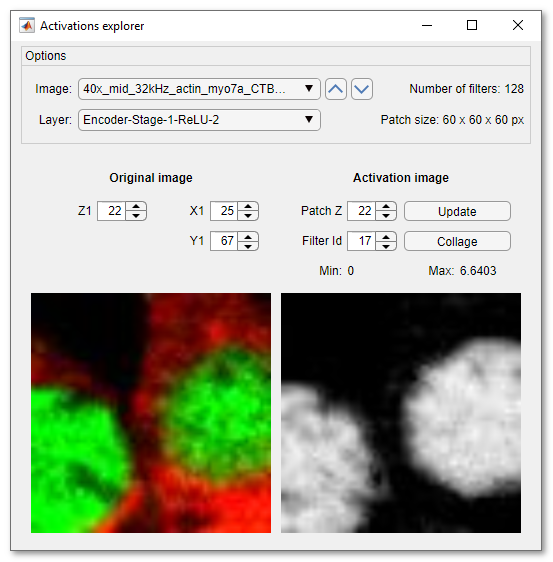
Here is the description of the options:
- Image ▼ has a list of all preprocessed images for prediction.
Selection of an image in this list will load a patch, which is equal to
the input size of the selected network
The arrows on the right side of the dropdown can be used to load previous or next image in this list - Layer ▼ contains a list of all layers of the selected network. Selection of a layer, starts prediction and acquiry of activation images
- Z1..., X1..., Y1..., these spinners make it possible to shift the patch across the image. Shifting of the patch does not automatically update the activation image. To update the activation image press the Update button
- Patch Z..., change the z value within the loaded activation patch, it is used only for 3D networks
- Filter Id..., change of this spinner brings various activation layers into the view
- Update press to calculate the activation images for the currently displayed patch
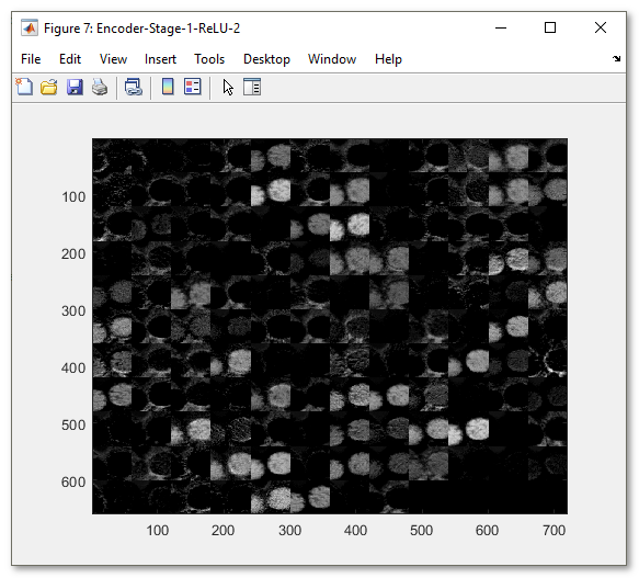
- Collage press to make a collage image of the current network layer activations
Snapshot with the generated collage image
Preview results section

- Load images and models press this button after finishing prediction to open original images and the resulting segmentations in the currently active buffer of MIB
- Load models press this button after finishing prediction to load the resulting segmentations over already loaded image in MIB
- Load prediction scores press to load the resulting score images (probabilities) into the currently active buffer of MIB
- Evaluate segmentation. When the datasets for prediction are accompanied with ground truth labels ( requires a label file(s) in the Labels directory under Prediction images directory; it is important that the model materials names match those for the training data!).
Details of the Evaluate segmentation operation
- Press the button to calculate various precision metrics

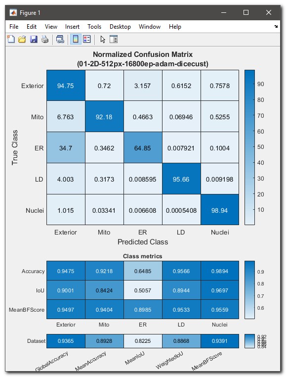
- As result of the evaluation a table with the confusion matrix will be
shown. The confusion matrix displays how well the predicted classes are
matching classes defined in the ground truth labels. The values are
scaled from 0 (bad) to 100 (excelent).
In addition, the calculated class metrics (Accuracy, IoU, MeanBGScore) as well as the global dataset metrics are shown.
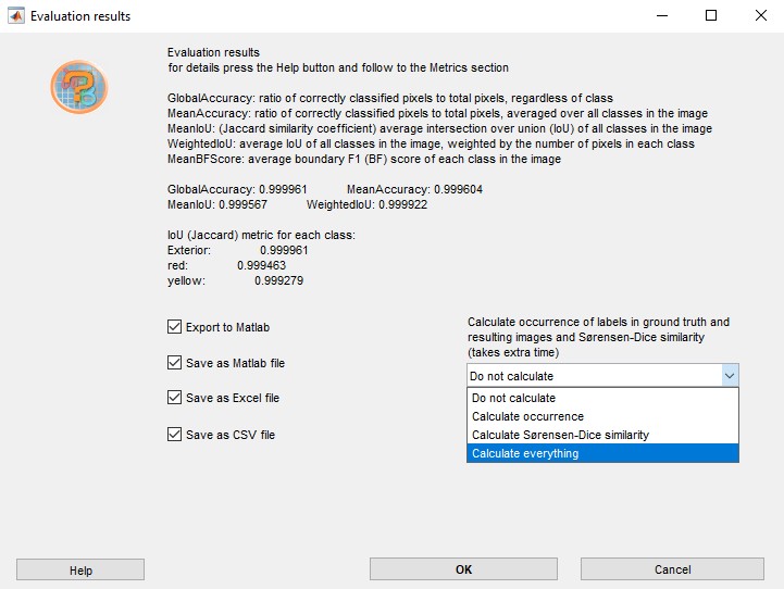
- In addition, it is possible to calculate occurrence of labels and Sørensen-Dice similarity coefficient in the
generated and ground truth labels. These options are available from a
dropdown located in the right-bottom corner of the Evaluation
results window:
- The evaluation results can be exported to MATLAB or
saved in MATLAB, Excel or CSV
formats to 3_Results\PredictionImages\ResultsModels directory, see more in the
Directories and Preprocessing section.
For details of the metrics refer to MATLAB documentation for evaluatesemanticsegmentation function
Back to Index --> User Guide --> Menu --> Tools Menu --> Deep learning segmentation