Image Menu
Image processing functions
Back to Index --> User Guide --> Menu
Contents
-
Mode -
Adjust Display/Image -
Color Channels -
Contrast -
Invert image -
Image filter -
Tools for images --> Content-aware fill -
Tools for images --> Debris removal -
Tools for images --> Image arithmetics (MIB for MATLAB only) -
Tools for images --> Intensity projection -
Tools for images --> Select image frame -
Tools for images --> White balance correction -
Morphological operations -
Intensity profile

Mode
Allows to change mode and color depth of the shown dataset
The following options are available
- Grayscale, converts image to grayscale by removing any color information
- RGB Color, converts image to the RGB color space
- HSV Color, converts image to the HSV (hue, saturation, value) color space
-
Indexed, converts image to the indexed colors (
not implemented for True Color images) -
8 bit, convert dataset to the 8 bit format, the image intensities are scaled to preserve the adjusted from the
View Settings Panel->Display dialog - 16 bit, convert dataset to the 16 bit format, the image intensities are scaled to preserve contrast of the original dataset
- 32 bit, convert dataset to the 32 bit format, the image intensities are scaled to preserve contrast of the original dataset
Adjust Display/Image
Starts a dialog to adjust display settings or resample image intensities. See more in the Adjust display window section
Color Channels
Perform some actions with color channels of the image
A brief demonstration is available in the following videos:- General demonstration:
 https://youtu.be/gT-c8TiLcuY
 - Correction of color shifts between images:
https://youtu.be/-J2P8a_z7pE
List of operations with color channels
- Insert empty channel..., insert an empty channel (intensity of all pixels is 0) to the specified position
- Copy channel..., copy one channel to another position
- Invert channel..., invert intensities of the specified color channel
- Rotate channel..., rotate the specified color channel
- Shift channel..., allows to shift a channel by X and Y pixels
- Swap channels..., allows to swap two color channels between each other
- Delete channel..., deletes specified color channel from the dataset
It is also possible to do color channel operations from the Colors table in the View settings panel.
Contrast
Adjust contrast of the dataset. For the linear contrast stretching it is recommended to use Image Adjustment dialog available via the Display button in the View Settings panel.
A tutorial on image normalization is available in the following video:
https://youtu.be/MmBmdGtuUdM
List of contrast adjustment operations
- Linear contrast, is no longer available in MIB, please use the Display button in the View Settings panel.
-
Contrast-limited adaptive histogram equalization, CLAHE contrast equalization. CLAHE operates on small regions in the image, called tiles, rather than the entire image. Each tile's contrast is enhanced, so that the histogram of the output region approximately matches the histogram specified by the 'Distribution' parameter. The neighboring tiles are then combined using bilinear interpolation to eliminate artificially induced boundaries. The contrast, especially in homogeneous areas, can be limited to avoid amplifying any noise that might be present in the image. For details see documentation for MATLAB function
adapthisteq. - Normalize layers, normalization of image intensities between the slices. A) calculates mean intensity and standard deviation (std) for the whole dataset; B) calculates mean intensities and standard deviation for each image; C) shifts each image based on difference between mean values of that image and the whole dataset, plus stretches it based on ratio between standard deviation of the whole dataset and each image. For the 4D datasets it is possible to perform normalization also via the time dimension. For the Z stack it is possible to exclude black or white pixels from consideration
- Normalize layers based on masked areas, essentially similar to the Normalize layers mode, except that all values are calculated from the masked areas only.
- Normalize based on masked background, normalizes image intensities between the slices using background areas that should be masked. A) calculates mean intensity for the masked area for the whole dataset; B) calculates mean intensities for the masked area for each image; C) shifts each image based on difference between mean values of the image and the whole dataset
Invert image
Invert image intensities, shortcut Ctrl+i|
A brief demonstration is available in the following video:
https://youtu.be/1DG2w5XYA18
Invert operations available for
- Shown slice (2D), invert only the currently shown slice of the dataset
- Current stack (3D), invert the current stack of the dataset
- Complete volume (4D), invert complete dataset
Image filter
Open a dialog with various image filters arranged into 4 categories:
- Basic image filtering in the spacial domain
- Edge-preserving filtering
- Contrast adjustment
- Image binarization
For further details, please refer to the Image Filters help page.
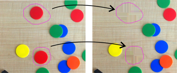
Tools for images --> Content-aware fill
Content aware fill can be used to reconstruct selected areas using information for neighboring regions.
A brief demonstration is available in the following video:
https://youtu.be/H_TVvgA_br4
Details of content-aware methods
 |
inpaintCoherentonly for MATLAB R2019a and newerRestore specific image regions using coherence transport based image inpainting. The areas for the content-aware fill can be specified using the Mask or Selection layers of MIB.
[1] F. Bornemann and T. M?rz. "Fast Image Inpainting Based on Coherence Transport." Journal of Mathematical Imaging and Vision. Vol. 28, 2007, pp.259?278. |
 |
inpaintExemplaronly for MATLAB R2019b and newerFill image regions using exemplar-based image inpainting The areas for the content-aware fill can be specified using the Mask or Selection layers of MIB.
[1] A. Criminisi, P. Perez and K. Toyama. "Region Filling and Object Removal by Exemplar-Based Image Inpainting." IEEE Trans. on Image Processing. Vol. 13, No. 9, 2004, pp. 1200?1212. |
Tools for images --> Debris removal
Automatically or manually restore areas of volumetric datasets that are corrupted with debris. The areas can either be automatically detected or manually selected into the Mask or Selection layers<br><br>
A brief demonstration is available in the following video:
https://youtu.be/iM2nHBxTjRw
Snapshot and details


|
|
Tools for images --> Image arithmetics (MIB for MATLAB only)
Use MATLAB syntax to apply custom arithmetic expression to Image, Model, Mask or Selection layers, see more in
a brief video and examples below.
For MIB 2.60 and newer
https://youtu.be/sDwvnJGLi8Q
For MIB 2.52 and older https://youtu.be/-puVxiNYGsI
Snapshot and details
 |
|
Examples of arithmetic operations
- I = I * 2, increase intensity of all pixels of the current image in 2 times
- I2 = I2 + 100, increase intensity of all pixels in image 2 by 100
- I1 = I1 + I2, add image from container 2 to an image in container 1 and return result back to container 1
- I3 = I3 + mean(I3(:)), add mean value of image 3 to image 3
- I1 = I1 - min(I1(:)), decrease intensity of pixels in the image 1 by the min value of the dataset
- I(:,:,2,:) = I(:,:,2,:)*1.4, increase image intensity of the second color channel in 1.4 times
- I(I==0) = I(I==0)+100, increase image intensity of the black areas by 100 intensity counts
- disp(sum(abs(single(I1(:))-single(I2(:))))), find the difference between two images loaded to container 1 and 2 and print it to console; or use msgbox(num2str()) instead of disp to show result as a message box
- M2 = M1, copy mask layer from image 1 to image 2
- for z=1:size(I, 4)
slice = I(:,:,2,z);
mask = M(:,:,z);
slice(mask==1) = 0;
I(:,:,2,z) = slice;
end - replace intensity of the second color channel in the masked area to 0
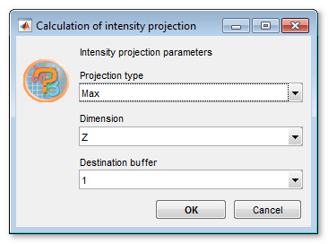
Tools for images --> Intensity projection
Generate intensity projection actoss any dimension of the loaded dataset
 |
A brief demonstration is available in the following video:
https://youtu.be/hwFpS_3eP9U
|
List of available projection calculations
-
Calculate one of the following intensity projections:
- maximum intensity projection, project the voxel with the highest value on every view throughout the volume onto a 2D image
- minimum intensity projection, project the voxel with the smallest value on every view throughout the volume onto a 2D image
- mean intensity projection, project the mean value of voxels on every view throughout the volume onto a 2D image
- median intensity projection, project the median value of voxels on every view throughout the volume onto a 2D image
- focus stacking, Generate extended depth-of-field image from focus sequence using noise-robust selective all-in-focus algorithm (Pertuz et. al. "Generation of all-in-focus images by
noise-robust selective fusion of limited depth-of-field
images" IEEE Trans. Image Process, 22(3):1242 - 1251, 2013)
Tools for images --> Select image frame
Detects the frame (which is an area of the same intensity that touches edge of the image) of the image. The detected area can be assinged to the Selection or Mask layers, or that area can be replaced with another color for the Image layer. |
A brief demonstration is available in the following video:
https://youtu.be/sWjipmeU5eA
|
Tools for images --> White balance correction
White balance correction demo
Correct white balance of the open dataset. Start with selection of an
area that should be white or gray and assign that to the Mask or
Selection layers or alternatively use the Manual mode and provide an RGB value
that should be corrected to become white or gray.
Snapshot, details and reference
 |
| For details please check chromadapt function |
|
Reference
[1] Lindbloom, Bruce. Chromatic Adaptation. http://www.brucelindbloom.com/index.html?Eqn_ChromAdapt.html |
Morphological operations
This section contains number of morphological operations that can be applied to images. The processed image may be also added or subtracted from the existing image (see the settings in the Additional action to the result panel).
A brief demonstration is available in the following video:
https://youtu.be/itbVLFm0FKQ
Snapshot
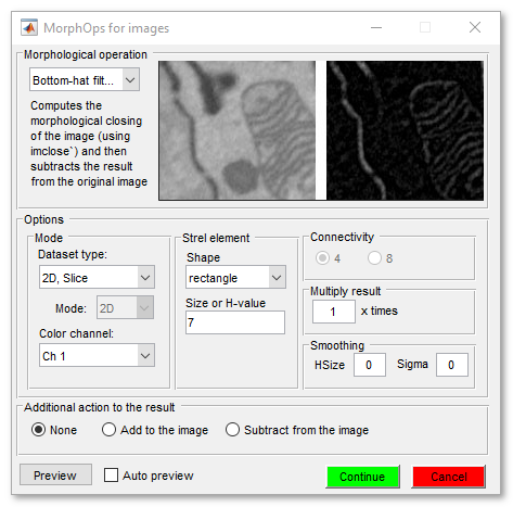
List of available morphological operations
- Bottom-hat filtering (imbothat) computes the morphological closing of the image (using imclose`) and then subtracts the result from the original image
- Clear border (imclearborder) suppresses light structures connected to image border
- Morphological closing (imclose) morphologically closes the image: a dilation followed by an erosion
- Dilate image (imdilate)
- Erode image (imerode)
- Fill regions (imfill) fills holes in the image, where a hole is defined as an area of dark pixels surrounded by lighter pixels
- H-maxima transform (imhmax) suppresses all maxima in the image whose height is less than H
- H-mminima transform (imhmin) uppresses all minima in the image whose depth is less than H
- Morphological opening (imopen) morphologically opens image: an erosion followed by a dilation
- Top-hat filtering (imtophat) computes the morphological opening of the image (using imopen) and then subtracts the result from the original image
Intensity profile
Generate an intensity profile of the image data. The profiles can be obtained in two modes:
- Line
- Arbitrary
For intensity profiles it is recommended to use the Measure length tool.
Back to Index --> User Guide --> Menu