Segmentation Tools
This panel hosts different tools that are used for the image segmentation. These tools are designed to help you separate and identify different regions or objects within an image.
Back to Index --> User Guide --> Panels --> Segmentation Panel
Contents
-
The 3D ball -
The 3D lines -
Annotations -
The Brush tool -
The Black and White Thresholding tool -
Drag & Drop material -
The Lasso tool -
The Magic Wand + Region Growing tool -
The Membrane Click Tracker tool -
Object Picker -
Segment-anything model -
The Spot tool
The 3D ball

|
The 3D ball tool is a segmentation tool that allows you to make a
selection in the form of a spherical object in a 3D space.
To use the "3D ball" tool, you need to specify the radius of the spherical object. The radius is taken from the Radius, px edit box, which allows you to define the size of the sphere. The larger the radius, the larger the selection will be. Additionally, there is an Eraser, x edit box that modifies the increase of the 3D ball eraser. This means that when you hold the ^ Ctrl key and use the eraser, the size of the eraser will increase based on the value specified in the Eraser, x edit box. A brief demonstration is available in the following video:  MIB in brief: Manual segmentation tools (https://youtu.be/ZcJQb59YzUA?t=1s)
Note! The aspect ratio for the depth size of the 3D ball is defined by the pixel dimensions, see Dataset Parameters in Menu->Dataset->Parameters |
Selection modifiers
- None / ⇧ Shift+left mouse click, add 3D ball selection with the existing one
- Ctrl + left mouse click, remove 3D ball selection from the current selection layer
The 3D lines
|
The "3D lines" tool is a powerful tool that allows you to draw lines in a
3D space and arrange them as graphs or skeletons.
The 3D lines are composed of nodes (vertices) that are connected with edges (lines that connect two nodes). These nodes and edges form the basis of the graph or skeleton structure. The nodes represent specific points or locations in the 3D space, while the edges represent the connections or relationships between these points. The 3D lines can be organized into separate trees, where each tree represents a distinct set of 3D lines. This allows for better organization and management of complex structures. A demonstration is available on:
Use of 3D lines for skeletons and measurements (https://youtu.be/DNRUePJiCbE)
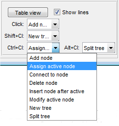
To modify the nodes in the 3D lines, you can use mouse clicks. The tool provides flexibility by allowing you to extend the mouse clicks with key modifiers such as ⇧ Shift, ^ Ctrl, and Alt. These key modifiers can be used to perform different actions or operations on the nodes, depending on your needs. Each action can be configured depending on needs. Please refer to a table below for various options. |
Available actions
- Add node ▼, add a new node to the active tree. This will create a new point in the 3D space and connect it to the active point (shown in red) of the tree. The new node will become part of the active tree
- Assign active node ▼ allows you to assign the closest node to the position of the mouse click as the new active node. This can be useful when you want to change the active node to perform specific operations or modifications
- Connect to node ▼, connects active node to another existing node. This will create an edge between the active node and the selected node, establishing a connection between them
- Delete node ▼, this will remove the closest node to the position of the mouse click. The edges of the tree will be rearranged to prevent splitting of the tree
- Insert node after active ▼, allows you to insert a new node after the active node. This can be useful when you want to add a new node in a specific position within the tree
- Modify active node ▼, this will allow you to move the active node to a new position in the 3D space using a mouse click
- New tree ▼, add a new node and assign it to a new tree. This new tree will not be connected to any other trees, providing a separate structure
- Split tree ▼, if you want to split a tree at a specific point, you can use the Split tree option. This will delete the closest node to the position of the mouse click and split the tree at that point.
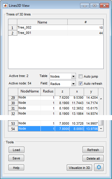
Press the Table view button to open a window that displays tables describing the 3D lines. This can provide additional information and details about the structure of the lines (see below).
Lines 3D View
|
Table with the list of trees
The upper table in the Lines 3D View window shows the list of trees and the number of nodes that compose each tree. It is important to note that each tree should have a unique name To access additional options for a tree, you can right-click on it. This will open a popup menu with various options:
|
Space between the tables
- Active tree, an index of the active tree
- Active node, an index of the active node
- The Table ▼ dropdown can be used to select what should be shown in the lower table below: Nodes or Edges
- The Field ▼ dropdown can be used to define an additional field that should be added to the lower table. By default, only the Radius and Weights fields are available
- [✓] Auto jump, when selected, auto jump to the selected node and show it in the Image View panel.
- [✓] Auto refresh, automatically refresh the tables, may be quite slow with many nodes
The Nodes table
The table shows list of nodes and offers multiple actions via a popup menu:
- Jump to the node ▼, jumps to the selected node and put it in the center of the Image View panel
- Set as active node ▼, makes the selected node active
- Rename selected nodes... ▼, assign a new name for the selected nodes
- Show coordinates in pixels... ▼, by default, the coordinates of the nodes are shown in the physical units of the dataset, i.e. with respect to the bounding box ; this action shows coordinate of the node in pixels
- New annotations from nodes ▼, generate a new annotations from the position of nodes
- Add nodes to annotations ▼, add selected nodes to the existing annotations
- Delete nodes from annotations ▼, delete selected nodes from the existing annotations
- Delete nodes... ▼, delete selected nodes
The Edges table
The table shows list of edges; certain actions available via a popup menu:
- Jump to the node ▼, jumps to the selected node and put it in the center of the Image View panel
- Set as active node ▼, makes the selected node active
Tools panel
- Load, load 3D lines from a file in MATLAB-compatible lines3d format
- Save, export to MATLAB or save 3D lines to a file:
- MATLAB format, *.lines3d, it is recommended to save the 3D lines in the matlab format!
- Amira Spatial graph, *.am, Amira-compatible format in binary or ascii form
- Excel format, *.xls, export Nodes and Edges tables to an Excel file
- Refresh, refresh the tables shown in this window
- Delete all, delete all 3D lines
- Visualize in 3D, plot all trees in the 3D space
- Settings, modify color and thickness of 3D lines
Annotations
|
A set of tools to add/remove annotations. Each annotation allows to mark
specific location in the dataset, assign a label and a value to it
Brief demonstration is available in the following videos: MIB in brief: Annotations (https://youtu.be/3lARjx9dPi0)
MIB in brief: Annotations (https://youtu.be/6otBey1eJ0U)
Addition and removal of annotations
|
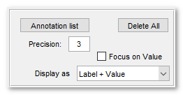
Annotation panel widgets
- The Annotation list button starts a window with the list of existing annotations. It is possible to load and save annotations to the main MATLAB workspace or to a file (matlab and excel formats). See more below.
- The Delete All button removes all annotations
- Precision edit box - specify number of digits after decimal point
- [✓] Show prompt checkbox, when ticked a dialog asking for label and value appear after addition of each annotation, otherwise the dialog is not shown and the label and field values are taken from the previously added annotation
- [✓] Focus on Value checkbox, when ticked, the first parameter during visualization of annotations is value and the second parameter is label.
- The Display as combobox - enables way how the annotations are
displayed in the Image View panel.
- The following modes are available:
- Marker, show only location of the annotation using a cross-marker
- Label, show marker and label for each annotation
- Value, show marker and value for each annotation
- Label + Value, show marker, label and value for each annotation
List of annotations window

|
|
|
|
The Brush tool

|
Use brush to make selection. The brush size is regulated with
the Radius, px edit box
A brief demonstration is available in the following videos: https://youtu.be/VlTCxVAUxFc
https://youtu.be/ZcJQb59YzUA?t=37s
Objects from different image slices may be connected using the Interpolation function (shortcut i or via Menu->Selection->Interpolate), see more in the Selection menu section. |
Controls
- ^ Ctrl + Mouse wheel, change brush size
- None / ⇧ Shift +
 left mouse click,
paint with brush
left mouse click,
paint with brush - ^ Ctrl + left mouse click, start eraser. The brush radius in the
eraser mode could be amplifier using the Eraser, x edit box.
- The [✓] auto fill checkbox in the Selection panel allows to perform automatic filling of areas after use of brush
Widgets of the brush panel
Radius, define radius of the brush tool in pixels
Eraser, x, define radius size multiplier when brush is in the eraser mode
Interpolation settings, press to start a dialog that allows to
modify the interpolation settings. The settings can also be modified from
the Preference dialog and the type can be switched
using a dedicated button in the toolbar.
 The [✓] Watershed checkbox, when ticked, pixels of the image are clustered using the watershed algorithm and can be selected as clusters (see the following section)
The [✓] SLIC checkbox, , when ticked, pixels of the image are clustered using the SLIC algorithm and can be selected as clusters (see the following section)
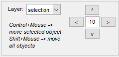
Superpixels with the Brush tool
The Superpixels mode can be initiated by selecting the Watershed or SLIC checkbox. In the Superpixels mode the brush tool selects not individual pixels but rather groups of pixels (superpixels). While drawing the selection of the last superpixel can be undone by pressiong the Ctrl+Z shortcut.
The superpixels are calculated using the
- SLIC (Simple Linear Iterative Clustering, good for objects with distinct intensities) algorithm written by Radhakrishna Achanta et al., 2015 , Ecole Polytechnique Federale de Lausanne (EPFL), Switzerland.
- Watershed (good for objects with distinct boundaries).
The two additional edit boxed (N, Compact/Invert) offer possibility to modify the size of generated superpixels (see below). The values in the N edit box can be changed using the Ctrl+Alt + mouse wheel or Ctrl+Alt+⇧ Shift + mouse wheel shortcuts.
References:
- Radhakrishna Achanta, Appu Shaji, Kevin Smith, Aurelien Lucchi, Pascal Fua, and Sabine S?sstrunk, SLIC Superpixels Compared to State-of-the-art Superpixel Methods, IEEE Transactions on Pattern Analysis and Machine Intelligence, vol. 34, num. 11, p. 2274 - 2282, May 2012.
- Radhakrishna Achanta, Appu Shaji, Kevin Smith, Aurelien Lucchi, Pascal Fua, and Sabine S?sstrunk, SLIC Superpixels, EPFL Technical Report no. 149300, June 2010.
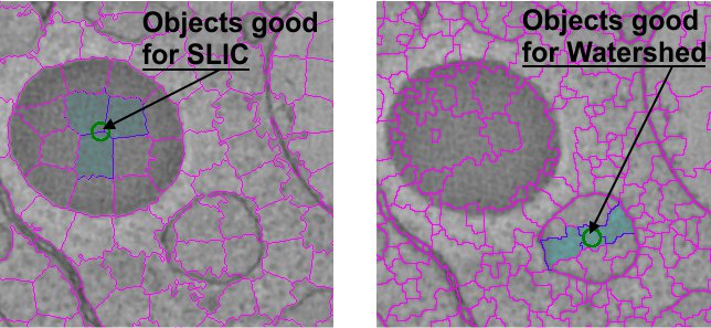
The set of superpixels is individual for each magnification (especially in the SLIC mode). It is possible to define size of superpixels (the N edit box, default value 220 for SLIC, for Watershed use lower numbers) and compactness (the Compact edit box; higher compactness gives more rectangularly shaped superpixels). In the Watershed mode the Compact edit box is called Invert; when objects have dark boundaries over bright backround number in the Invert edit box should be 1 (or higher), if the objects have bright boundaries over dark background this number should be 0.
During drawing the boundaries of the superpixels for the SLIC mode are shown using the drawregionboundaries.m function written by Peter Kovesi Centre for Exploration Targeting, School of Earth and Environment, The University of Western Australia.
Note 1! The Superpixels mode is sensitive to the [✓] Adapt. checkbox in the Selection panel. When the [✓] Adapt. checkbox is selected the superpixels are selected based on the mean value of the initial selection plus/minus standard deviation within the same area multiplied by the factor specified in the Adapt. editbox of the Selection panel.
Note 2! While drawing the value in the Adapt. editbox may be changed using the mouse wheel.
Note 3! The function relies on slicmex.c that should be compiled for your operating system. Please refer to the Microscopy Image Browser System Requirements section for details.
The Black and White Thresholding tool

|
Makes black and white thresholding of the current image slice or the
whole dataset (depending on status of the [✓] 3D and [✓] 4D checkboxes).
The black-and-white thresholding is initiated upon change of sliders,
modification of editboxes or by hittin Threshold
A brief demonstration is available in the following video: https://youtu.be/ZcJQb59YzUA?t=4m37s
|
Parameters and controls
Use the Low and High sliders and edit boxes to provide threshold values that will be used to select pixels with intensities between these values. The thresholding process is automatically initiated upon interaction with these widgets.
If the Masked area check box is selected the thresholding is performed only for the masked areas of the image, which is very convenient for local black and white thresholding.
Right mouse click above the threshold sliders opens a popup menu that allows to set precision for the slider movement.
The [✓] Adaptive checkbox starts adaptive threshoding with the Sensitivity and Width parameters modified by the scroll bars.
Usage notes
When doing thesholding for large 3D/4D datasets it is recommended to:
- start in 2D mode by unchecking [✓] 3D and [✓] 4D checkboxes
- adjust parameters using the currently shown slice
- when parameters are chosen, tick [✓] 3D or [✓] 4D checkbox
- Press the Threshold button to start black-and-white thresholding
Drag & Drop material
|
Shift MIB layers (selection, mask, model) to left/right/up/down
direction. The tool allows to move individual 2D/3D objects as well as
complete contents of the layers in 2D and 3D.
A combobox offers possibility to choose the layer to be moved. Mouse click or use of the buttons in the panel move the selected layer left/right/up/down by the specified number of pixels. A brief demonstration is available in the following video: https://youtu.be/NGudNrxBbi0
|
Mouse and key controls
| Start by | Modifier | [✓] 3D checkbox | Action |
| Left mouse click over an object | Ctrl | Unchecked | Move the selected object in 2D |
| Left mouse click over an object | Ctrl | Checked | Move the selected 3D object. Note! Only for MATLAB version 2017b and newer |
| Left mouse click | ⇧ Shift | Unchecked | Move all objects on the shown slice, i.e. 2D movement |
| Left mouse click | ⇧ Shift | Checked | Move all objects on all slices, i.e. 3D movement |
| Left/Right/Up/Down buttons | - | Unchecked | Move all objects on the shown slice by the specified number of pixels, i.e. 2D movement |
| Left/Right/Up/Down buttons | - | Checked | Move all objects on all slices by the specified number of pixels, i.e. 3D movement |
The Lasso tool
|
Selection with a lasso, rectangle, ellipse or polyline tools.
A brief demonstration is available in the following video: https://youtu.be/OHFdGj9uBro
|
How to use:
- Press and release left mouse button above the image to initialize the lasso tool
- Press and hold left mouse button and drag the mouse to select an area
- Release the left mouse button to finish the selection process
- Modify selected area, if needed
- Accept selection using double left mouse button click
Modes:
- Add, a new selection is added to the existing one
- Subtract, a new selection is subtracted from the existing one
The Lasso tool works also in 3D.
The Magic Wand + Region Growing tool
|
Selection of pixels with the _mouse button_ based on their
intensities. The intensity variation is calculated from the intensity of the
selected pixel and two threshold values from the |Variation| edit boxes.
A brief demonstration is available in the following video: https://youtu.be/ZcJQb59YzUA?t=1m50s
|
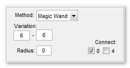
Widgets and parameters
- Variation editboxes, specify variation of image intensities relative to the clicked value
- Connect 8 specifies the 8 (26 for 3D) connected neighbourhood connectivity
- Connect 4 specifies the 4 (6 for 3D) connected neighbourhood connectivity
- Radius allows defining an effective range for the magic wand
The Magic Wand works also in the 3D mode (the 3D switch in the Selection panel).
Selection modifiers for the Magic wand tool
- left mouse click, will replace the existing selection with the new one.
- ⇧ Shift + left mouse click, will add new selection to the existing one.
- Ctrl + left mouse click, will remove new selection from the current.
The Membrane Click Tracker tool
|
This tool tracks membrane-type objects by using 2 mouse clicks that define start and end point of the membrane domain.
A brief demonstration for 2D is available in the following video: https://youtu.be/ZcJQb59YzUA?t=3m14s
A brief demonstration for 3D is available in the following video: https://youtu.be/ZcJQb59YzUA?t=2m22s
|
How to use
- Ctrl + left mouse click to define the starting point of a membrane fragment (before MIB version 2.651 the ⇧ Shift + left mouse click combination was used)</li>
- Left mouse click to trace the membrane from the starting point to the clicked point</li>
Additional parameters
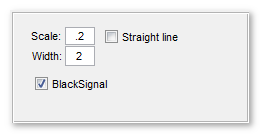
- The Scale edit box - during the tracing the image gets enhanced by taking into account intensities of the starting and ending points
img(img>min([val1 val2])-diff([val1 val2])*options.scaleFactor) = maxIntensity; - The Width edit box - defines a width of the resulting trace
- The [✓] BlackSignal checkbox defines whether the signal is Black on White, or White on Black
- The [✓] Straight line checkbox - when checked, the points are connected with a straight line
Note! When the 3D switch in the Selection panel is enabled the Membrane Click Tracker tool connects points (linearly) in the 3D space (this may be very usefull for tracing microtubules). Alternatively for microtunules, consider
Reference and compilation
The membrane is traced with help of Accurate Fast Marching function http://www.mathworks.se/matlabcentral/fileexchange/24531-accurate-fast-marching by Dirk-Jan Kroon, 2011, University of Twente.
Note! It is highly recommended to compile the corresponding function (see details in the Membrane Click Tracker section of the System Requirements page ), otherwise the function is very slow!
Object Picker
|
This mode allows fast selection of objects from the Mask or
Model layers depending on what row is selected in the segmentation table.
A brief demonstration is available in the following video: https://youtu.be/mzILHpbg89E
Works also in 3D (select the 3D check box in the Selection panel). Note! The 3D mode requires calculating statistics for the objects. Please select the material in the Select from list box and press the Recalculate stats for 3D objects button (the button becomes available when the Mask->Mask statistics... or Menu->Models->Model statistics.... |
Possible Object Picker selection modes
-
1. Left mouse click, selects object from the Mask/Model layers with a single mouse click.
Note 1! Separation of objects is sensitive to the connected neighbourhood connectivity parameter from the Magic Wand tool; Note 2! In the 3D mode the function uses object statistics that is generated by pressing the Recalc. Stats button. If the Mask/Model layers have been changed press the Recalc. Stats button again. -
2. Lasso: selects object with lasso tool (Press first
None/⇧ Shift/Ctrl + Right mouse button,
then hold the left mouse button while moving mouse around). Can also make selection for the whole dataset if the [✓] 3D checkbox in
the Selection panel is checked.
- 3. Rectangle or Ellipse: these tools work in similar to the lasso tool manner but give rectangle or ellipsoid selection. Works also in 3D.
-
4. With the Polyline option the selection is done by drawing a polygon
shape point by point. Start drawing with the right mouse button and finish with
a double click or the
 right mouse click. Works also in 3D.
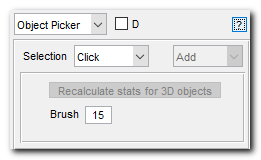
- 5. Use Brush to select some of the masked/model areas. Size of the Brush tool is defined in the Brush editbox.
-
6. Mask within selection with the left mouse click on the image
make a new selection that is an intersection of the existing selection
and the mask/model layer. With Ctrl+ mouse click the new selection is
Selection -minus- Mask. This action is sensitive to the [✓] 3D checkbox state in the Selection panel.
Selection modifiers
- None/⇧ Shift + left mouse click, will add selection with the existing one
- Ctrl + left mouse click, will remove selection from the current
Segment-anything model

|
Use Segment-anything model (SAM1 or SAM2) for object segmentation using one or few mouse clicks
An extensive tutorial covering installation and usage (SAM1): https://youtu.be/J3pivV4udGU
|
General information and reference
- SAM-1: https://segment-anything.com
- SAM-2: https://ai.meta.com/sam2/
Implementation of SAM in MIB is done via utilization of an external Python interpreter, please check the Requirements and installation section below for detailed instructions.
Important! even though SAM can work on CPU, GPU is highly recommended as it is x30-60 faster.
List of original SAM-1 available in MIB:
- vit_b (0.4Gb), fastest (x1) but gives less precise results
- vit_l (1.2Gb), moderate speed (~x1.4 slower), better predictions
- vit_h (2.5Gb), slowest (x2.0 slower), best predictions
-
Alexander Kirillov, Eric Mintun, Nikhila Ravi, Hanzi Mao, Chloe Rolland, Laura Gustafson, Tete Xiao, Spencer Whitehead, Alexander C. Berg,
Wan-Yen Lo, Piotr Dollar, Ross Girshick
Segment Anything arXiv:2304.02643, https://doi.org/10.48550/arXiv.2304.02643
- vit_b Electron Microscopy (0.4Gb), the lightest implementation for fast response of SAM trained on electron microscopy datasets
- vit_b Light Microscopy (0.4Gb), the lightest implementation for fast response of SAM trained on light microscopy datasets
- vit_h Electron Microscopy (2.5Gb), the extensive implementation for best results of SAM trained on electron microscopy datasets
- vit_h Light Microscopy (2.5Gb), the extensive implementation for best results of SAM trained on light microscopy datasets
- vit_b for EM Generalist (0.4Gb), pretrained for detection of mitochondria from EM datasets
- vit_b for EM Boundaries (0.4Gb), pretrained for detection of membrane encapsulated organelles from EM datasets
-
Anwai Archit, Sushmita Nair, Nabeel Khalid, Paul Hilt, Vikas Rajashekar, Marei Freitag, Sagnik Gupta, Andreas Dengel, Sheraz Ahmed, Constantin Pape
Segment Anything for Microscopy, bioRxiv, doi: https://doi.org/10.1101/2023.08.21.554208; link
- sam2_hiera_tiny (0.15Gb)
- sam2_hiera_small (0.18Gb)
- sam2_hiera_base_plus (0.32Gb)
- sam2_hiera_large (0.90Gb)
-
Nikhila Ravi, Valentin Gabeur, Yuan-Ting Hu, Ronghang Hu, Chaitanya Ryali, Tengyu Ma, Haitham Khedr,
Roman Rädle, Chloe Rolland, Laura Gustafson, Eric Mintun, Junting Pan, Kalyan Vasudev Alwala,
Nicolas Carion, Chao-Yuan Wu, Ross Girshick, Piotr Dollar, Christoph Feichtenhofer
SAM 2: Segment Anything in Images and Videos
arXiv:2408.00714, https://arxiv.org/abs/2408.00714
Download links and configuration file
SAM networks are automatically connected to MIB; it is possible to configure any custom SAM network for use in MIB. To do so, please modify sam_links.json for SAM-1 and sam2_links.json for SAM-2 located by default under Resources subfolder within MIB. It is also possible to link this file from anywhere, in this case use segment-anything settings in MIB to provide a new location.
Requirements and installation instructions
Installation details:
How to use
Interactive
It is a default operation mode of SAM in MIB. In this mode the segmentation is performed on the part of the image that is visible to the user. To start segmentation do following:- Use the Destination ▼ dropdown to define the destination layer: selection, mask, model. Depending on this, the results of the segmentation procedure are automatically assigned to the selected layer
- Use the Mode ▼ dropdown to define the operation that needs to
be applied to the segmentation results:
- Replace, replace the objects of the destination layer with the new segmentation results
- Add, add segmentation results to the objects of the selected destination layer
- Subtract, subtract segmentation results from the objects of the selected destination layer
- add, +next material, add segmentation results to the selected material and automatically add a new material to the model. This mode is only for models with 65535+ and when the destination layer is model or selection.
- Use left mouse click to specify a point on
the image that belongs to an object to be segmented.
If the object was not segmented with a single click:- ⇧ Shift + Left mouse click, expands the object
so that the new area under the click is added to the object
- Ctrl + Left mouse click
to deselect the selected area from the object
- ⇧ Shift +
Landmarks
This mode can be used to process full images. The idea that the key points are provided as annotations:- Use the Dataset ▼ dropdown to define portion of the image stack to process
- Use the Destination ▼ and Mode ▼ dropdowns to define destination layer and the mode (see the Interactive mode above for details)
- Use Left mouse click to add annotations.
The annotation value defines whether the annotation's location defines object (Value=1)
or background (Value=0)
- Hints:
- Hint 1: use Annotations ▼-> [✓] Focus on Value to focus the value instead of the annotation label
- Hint 2: uncheck Annotations ▼-> [✓] show prompt to switch off the dialog asking for annotation label and value
- Hint 3: use Ctrl + Left mouse click
to remove the closest to the mouse click annotation
- Hint 4: it is possible to access the list of annotation by pressing
- PressSegment to do segmentation
Automatic everything
In this mode, MIB is using SAM to segment all objects automatically and assigns them to a new model:- Use the the Dataset ▼ dropdown to define portion of the image stack to process
- PressSegment to do segmentation
SAM settings
 to open the settings
dialog.
to open the settings
dialog.
There are various settings that can be affected to finetune the segmetation process. Here the list of the most important parameters:
-
There are various settings that can be affected to finetune the
segmetation process. Here the list of the most important parameters
- Backbone ▼, define a pretrained backbone to be used. There are 7 backbones of different sizes, the larger the size - the longer it takes to get predictions, but the quality of the prediction is better. See the General information and reference section above for details
- Execution environment ▼, define whether GPU (the cuda mode) or CPU should be used. The CPU mode is significantly slower than the GPU mode
- [✓] Show the progress bar in the interactive mode, uncheck to switch off showing of the progress bar during segmentation
- PATH to segment-anything installation, location where segment-anything package was unzipped. You can click [✓] Check to select path to segment-anything to open a directory selection dialog to specify this folder
The Spot tool

|
Adds a spot - a circular object with a mouse click
A brief demonstration is available in the following video: https://youtu.be/AlCzjKuyJww
|
Widgets and parameters
*Eraser, x*, specifies magnifier for the spot eraser tool
Works also in 3D.
Selection modifiers
- None/⇧ Shift + left mouse click, will add new spot to the existing ones
- Ctrl + left mouse click, will remove selection from the current
Back to Index --> User Guide --> Panels --> Segmentation Panel