Deep MIB - Train Tab

Back to MIB | User interface | DeepMIB

Settings for generating and training deep convolutional networks in Microscopy Image Browser.

Overview

The Train tab in Deep MIB contains settings for designing and training deep convolutional networks. before starting, adjust the default settings to your project’s needs and ensure the output network file is specified using the Network filename button in the Network panel.

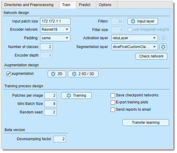
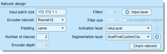
Network design

The Network design section configures the network architecture.

Network design section

Input patch size... defines the dimensions of image blocks (height, width, depth, colors) for training (e.g., "572 572 1 2" for a 572x572x1 patch with 2 color channels), Define the input patch size based on available GPU memory, desired field of view, dataset size, and channels. Patches are randomly sampled, with the count set in Patches per image...
Encoder network selects the encoder for supported architectures, sorted from lightweight to more complex
Padding sets convolution padding type:
- same: adds zero padding to keep input/output sizes equal
- valid: no padding, reducing output size but minimizing edge artifacts (though same with overlap prediction also reduces artifacts).

Info

Press Check network to verify compatibility of the input patch size with the selected padding method

Number of classes... specifies the total number of materials, including Exterior
Encoder depth... sets the number of encoding/decoding layers in U-Net, controlling downsampling/upsampling by 2^D. Tweak with Downsampling factor... (Beta version) to adjust patch size
Filters... defines the number of output channels (filters) in the first encoder stage, doubling per subsequent stage, mirrored in the decoder
Filter size... sets convolutional filter size (e.g., 3, 5, 7)
Input layer configures input image normalization settings
use ImageNet weights (MATLAB version only) initializes 2D patch-wise networks with ImageNet pretrained weights (ImageNet); requires corresponind supporting packages to be installed
Activation layer selects the activation layer type, with additional settings via the button when available

list of available activation layers

Compare activation layers here:
- reluLayer: Rectified Linear Unit (ReLU) layer, default activation layer
- leakyReluLayer: Leaky Rectified Linear Unit (ReLU) layer scales negative inputs
- clippedReluLayer: Clipped Rectified Linear Unit (ReLU) layer performs a threshold operation, where any input value less than zero is set to zero and any value above the clipping ceiling is set to that clipping ceiling
- eluLayer: Exponential linear unit (ELU) layer exponential nonlinearity for negatives
- swishLayer: Swish activation layer applies f(x) = x / (1+e^(-x))
- tanhLayer: Hyperbolic tangent (tanh) layer

Segmentation layer selects the output layer, with settings via the button when available

List of available segmentation layers

pixelClassificationLayer: cross-entropy loss
focalLossLayer: focal loss for class imbalance
dicePixelClassificationLayer: generalized Dice loss for class imbalance
dicePixelCustomClassificationLayer: modified Dice loss for rare classes

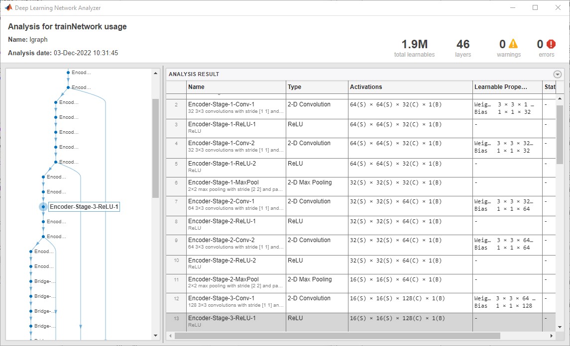
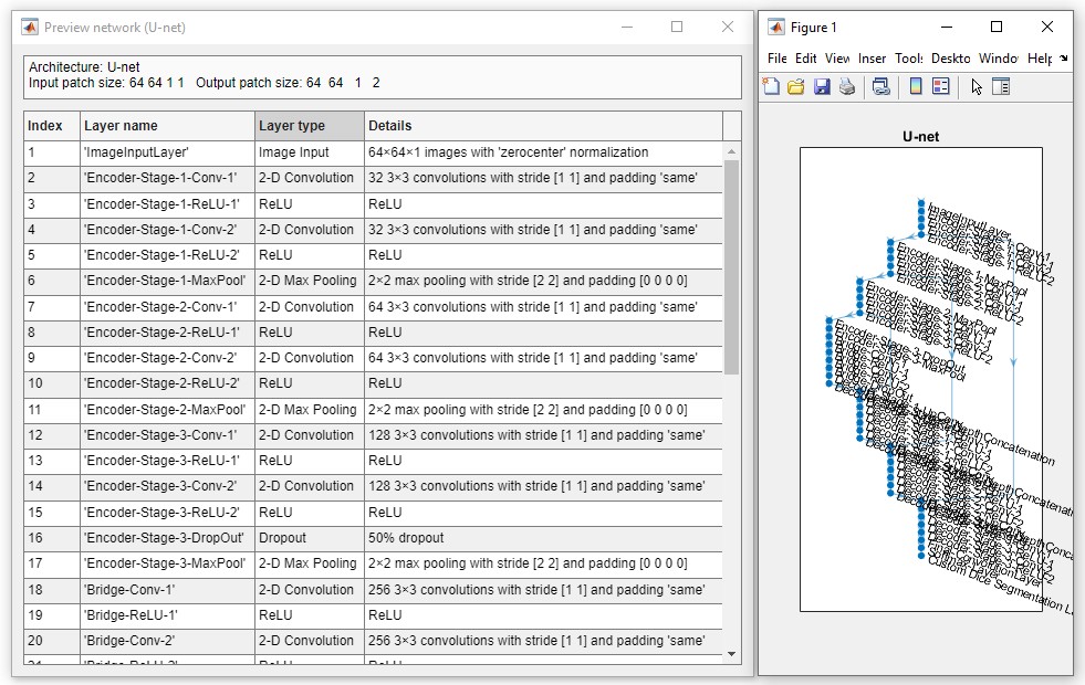
Check network previews and validates the network (limited info in standalone MIB)

Snapshots of the network check window for the MATLAB and standalone versions of MIB

MATLAB version:

Standalone version:

Augmentation design

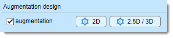
Augmentation enhances training data with image processing filters (17 for 2D, 18 for 3D networks), configurable via buttons next to Augmentation.

Augmentation: enables augmentation of input patches
2D: sets augmentation for 2D networks (17 operations)
3D: sets augmentation for 3D networks (18 operations)

Specify the fraction of patches to augment, plus probability and variation per filter. Multiple filters may apply to a patch based on probability.

2D/3D augmentation settings

Press 2D or 3D to open the settings dialog:

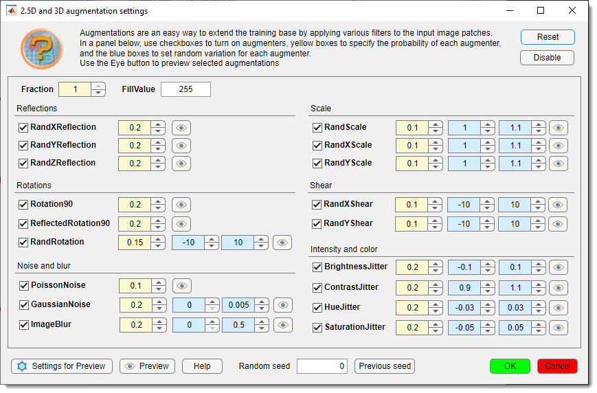
- Toggle augmentations with checkboxes
- Set probability (yellow) and variation (light blue)
- Reset restores defaults
- Disable turns off all augmentations
- Fraction probability of patch augmentation (1 = all, 0.5 = 50%)
- FillValue background color for downsampling/rotation (0 = black, 255 = white for 8-bit)
- Eye icon previews patches with augmentations, fixed or random based on Random seed (0 = random)
- Preview settings adjusts preview parameters

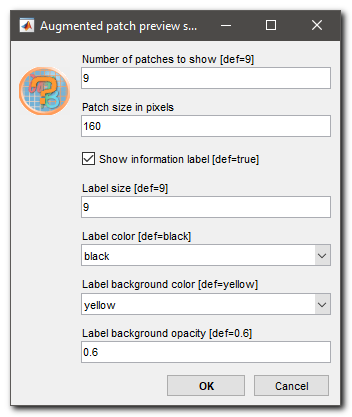
Details settings for preview

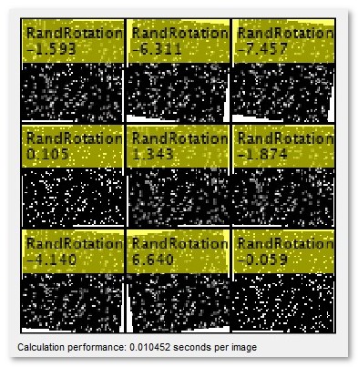
Example augmentations from Preview:

Help: links to training help
Previous seed: restores the last random seed (when Random seed = 0)
OK: applies settings
Cancel: discards changes

Training process design

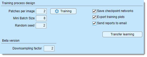
The Training process design section configures the training process, started with Train.

Patches per image... sets patches per image/dataset per epoch. Use 1 patch with many epochs and Shuffling: every-epoch (via Training) for best results, or adjust as needed
Mini Batch Size... number of patches processed simultaneously, limited by GPU memory. Loss is averaged across the batch
Random seed... seeds the random number generator for training initialization (use any fixed value except 0 for reproducibility, otherwise use 0 for random initialization each training attempt)
Training sets multiple parameters (see trainingOptions).

Tip

set Plots to "none" for up to 25% faster training

Save checkpoint networks saves checkpoints after each epoch to 3_Results/ScoreNetwork. Resume training from checkpoints via a dialog. In R2022a or newer, it is possible to adjust frequency for saving checkpoints
Export training plots saves accuracy/loss scores to 3_Results/ScoreNetwork in .score (MATLAB) and CSV formats, using the network filename
Send reports to email emails progress/finish updates. configure SMTP settings via the checkbox

Configuration of email notifications

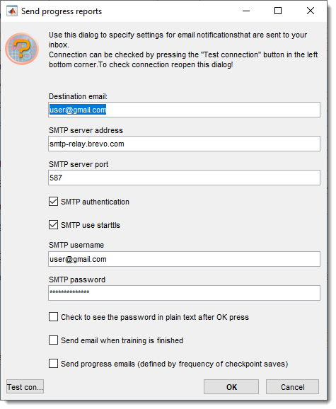
- Destination email recipient address
- STMP server address SMTP server address
- STMP server port server port
- STMP authentication enables authentication
- STMP use starttls enables TLS/SSL
- STMP username server username (e.g., Brevo email)
- STMP password server password (hidden, toggle Check to see the password in plain text after OK press to view) - Send email when training is finished emails on completion
- Send progress emails emails progress (custom training dialog only, frequency tied to checkpoints)
- Test connection tests settings after saving with OK

Important!

Important: Use dedicated SMTP services (e.g., Brevo) instead of personal email accounts

Configuration of brevo.com SMTP server

Sign up at Brevo
Access SMTP and API from the top-right menu:
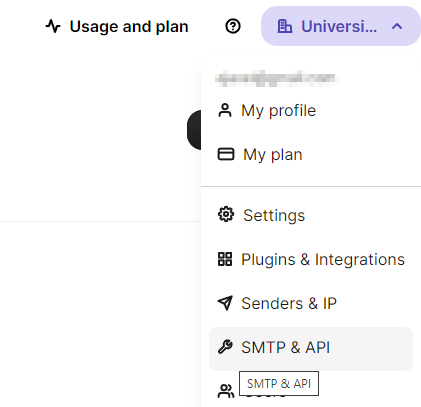
Click Generate a new SMTP key
Copy the key to the password field in email settings

Start the training process

Click Train to begin. If a network file already exists in Network filename..., a dialog offers to resume training.
A .mibCfg config file is saved in the same directory, loadable via Options tab → Config files → Load.

During training, a loss function plot appears (blue = training, red = validation), with accuracy gauges at the bottom left. Perform over the plot to scale it via a context menu.
Stop training with Stop or Emergency brake (faster but may not finalize networks with batch normalization).

By default, Deep MIB uses a custom progress plot. If you want to use default MATLAB’s training plot (MATLAB version only), uncheck Options tab → Custom training plot → Custom training progress window.
Disable plots for speed via Train tab → Training → Plots → none.
Preview patches (bottom right) reduce performance; adjust frequency in Options tab → Custom training plot → Preview image patches and Fraction of images for preview (1 = all, 0.01 = 1%).

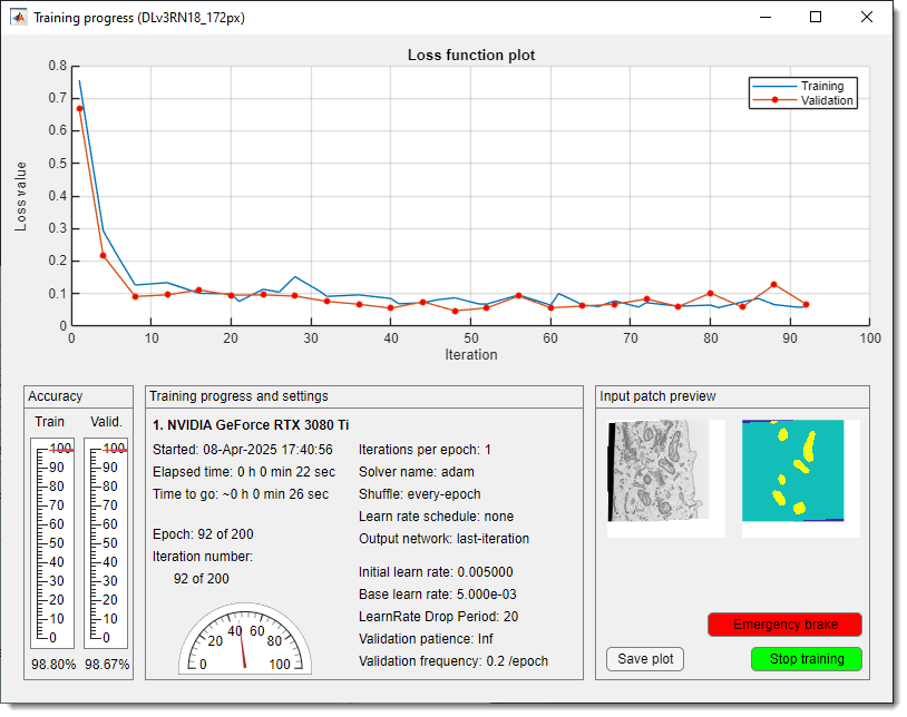
Training process window — Custom DeepMIB training loss plot

After training, the network and config files are saved to the location in Network filename....

Back to MIB | User interface | DeepMIB