Graphcut Segmentation
Back to MIB | User interface | Menu | Tools
Semi-automated image segmentation using the max-flow/min-cut graphcut method in Microscopy Image Browser (MIB).
Overview
The Graphcut segmentation tool in MIB provides semi-automated segmentation using the max-flow/min-cut algorithm. It is based on the Max-flow/min-cut algorithm by Yuri Boykov and Vladimir Kolmogorov, with a MATLAB implementation by Michael Rubinstein.
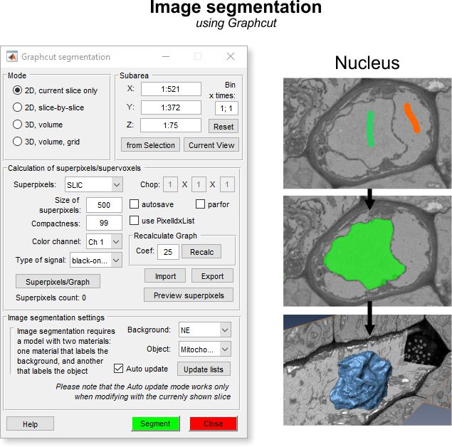
Instead of segmenting individual pixels, it operates on superpixels (2D) or supervoxels (3D),
generated via the SLIC algorithm by
Radhakrishna Achanta et al. or the Watershed algorithm. SLIC superpixels excel for
objects with intensity contrast, while Watershed superpixels are better for objects with
distinct boundaries.
Precomputing superpixels requires initial processing time but accelerates subsequent segmentation.
General example
A demonstration is available in this video:
Watch on YouTube
How to use
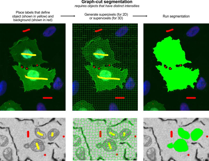
Steps to perform graphcut segmentation:
- Use two labels to mark background and object areas of interest
- Launch the tool via
Menu → Tools → Semi-automatic segmentation → Graphcut - Choose a mode: 2D or 3D
- Select superpixel/supervoxel type: SLIC or Watershed
- Generate superpixels/supervoxels by clicking
- Verify and adjust superpixel size if necessary
- Click to start segmentation
Note
Some functions may require compilation; see the System Requirements page for details
Mode panel
The Mode panel lets you select the segmentation scope.

- segments only the current slice in the Image View panel
- applies 2D segmentation to each slice individually
- performs 3D segmentation on the entire dataset or a subarea (see Subarea panel below)
- segments a large dataset by dividing it
into subvolumes (defined by Chop fields). the subvolume centered in
the Image View panel is processed
(enable the center marker via
 on the toolbar).
Use to process all subvolumes
Subarea panel
The Subarea panel defines a dataset subset for processing, useful for large datasets or binning.
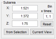
- sets the width range (e.g.,
1:512) - sets the height range
- sets the z-slice range
- fills X, Y, and Z with coordinates from the Selection layer’s bounding box
- limits X and Y to the visible area in the Image View panel
- restores full dataset dimensions
- applies a binning factor to reduce detail for faster processing
Warning
Auto update mode () is unavailable with binned datasets
Calculation of superpixels/supervoxels
Superpixels (2D) or supervoxels (3D) are precomputed using SLIC or Watershed algorithms. SLIC suits intensity-contrast objects (e.g., lipid droplets), while Watershed excels for boundary-defined objects.
Image example of clusters
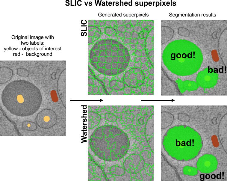
![]()
- selects the type: SLIC or Watershed
- sets approximate superpixel size (SLIC only)
- scaling factor defining size of superpixels (Watershed only)
- (1-99) controls superpixel squareness; higher values yield squarer shapes (SLIC only)
- chooses the color channel for superpixel calculation
- selects black-on-white (electron microscopy) or light-on-black (light microscopy)
- defines subvolume sizes for 3D volume grid mode or SLIC supervoxels
- saves the graphcut structure and supervoxels to disk automatically
- enables parallel processing for Watershed clustering in 3D volume grid mode, boosting performance
- uses supervoxel indices for final models, improving performance but requiring more memory
- generates superpixels and organizes them into a graph
- loads superpixels and graphs from disk or MATLAB
- saves superpixels and graphs to a file, MATLAB, a new model, or as a Lines3D graph object (not recommended for many superpixels; see this video)
- displays the generated superpixels
Image segmentation settings
The Graphcut workflow uses labeled areas (Background and Object) for segmentation, offering faster interaction than the Watershed workflow. It handles objects with both boundaries and intensity contrast, making it versatile.
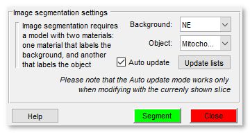
- selects the model material labeling background areas
- selects the model material labeling objects
- refreshes material lists
- updates segmentation automatically when materials change (best for small datasets, ~400x400x400 pixels)
Warning
In Auto update mode, use only the
shortcut (not ).
Recalculate final segmentation with
.
This mode is unavailable with binned datasets
Image segmentation example
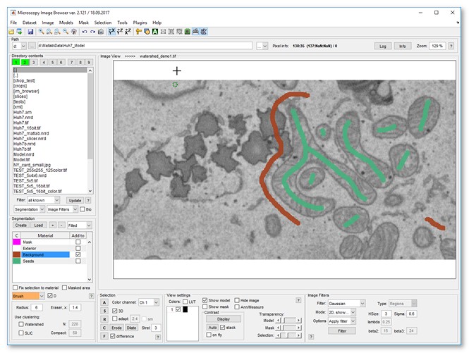
Follow these steps to segment mitochondria using Graphcut:
- Load a sample dataset:
Menu → File → Import image from → URL, enter http://mib.helsinki.fi/tutorials/WatershedDemo/watershed_demo1.tif - Add a material named Background in the Segmentation panel with (right-click to rename)
- Use the Brush tool to label cytoplasm, then press to add it to Background
Snapshot
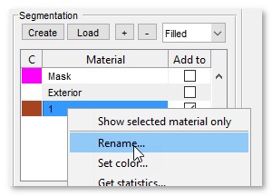
- Add another material named Seeds with
- Label mitochondria interiors, then press to add to Seeds
Snapshot
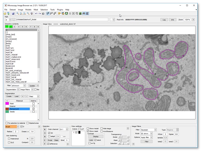
- Start Graphcut via Menu → Tools → Semi-automatic segmentation → Graphcut
- Select Watershed in
- Ensure Background and Seeds are set in Image segmentation settings
- Click to segment mitochondria
- Add more seeds to refine, then re-segment with or enable
- Results appear in the Mask layer
- Optionally smooth the mask: Menu → Mask → Smooth Mask
Snapshot
References
- Max-flow/min-cut algorithm by Yuri Boykov and Vladimir Kolmogorov (research license only)
- MATLAB wrapper for maxflow by Michael Rubinstein
- SLIC superpixels and supervoxels by Radhakrishna Achanta et al.
- Region Adjacency Graph (RAG) by David Legland, INRA, France (modified for Watershed)
Back to MIB | User interface | Menu | Tools